Transformers from Scratch

So, there are plenty of “Transformers from Scratch” articles and videos out there in the wild and I would be lying if I said I did not look at any of them before writing my own. So why this?

My motivation to share was purely just for demonstration as to how I wrote my own small module for transformers “from scratch”. This was useful exercise for me to understand the internals of the transformer architecture and build the necessary foundation for more complex LLM models.

To start with, let’s import the libraries and modules we will use.

import torch
from torch import nn
import math
from torch.utils.data import DataLoader, TensorDataset
from transformers import AutoTokenizer, AutoModel
from torch.nn import functional as F

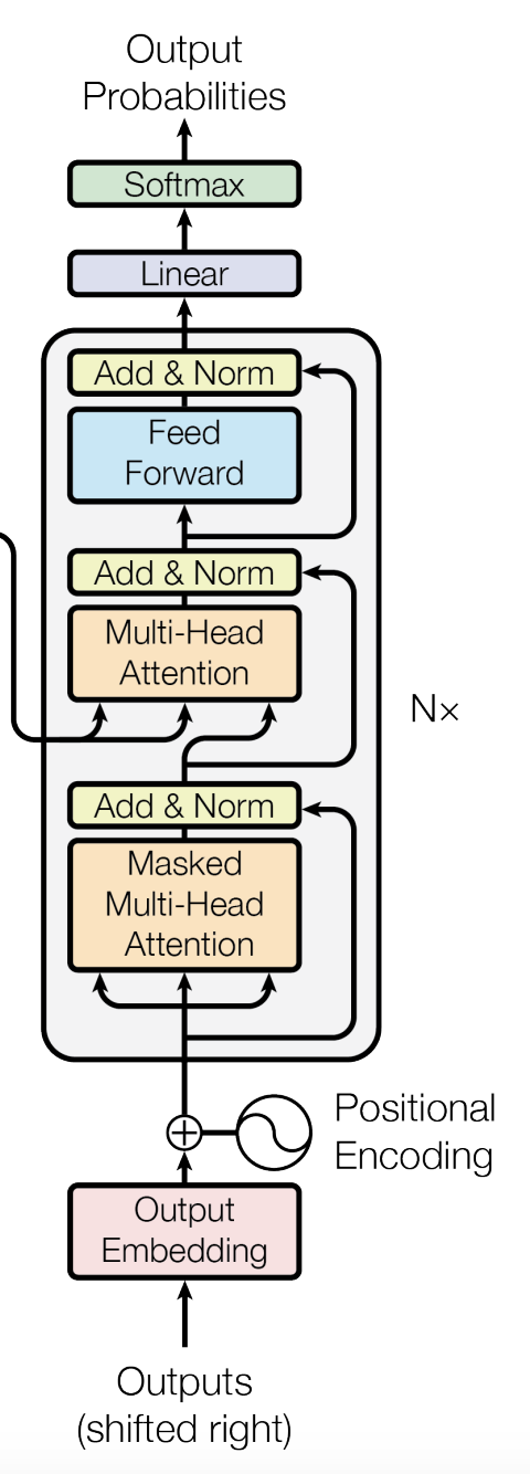
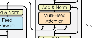
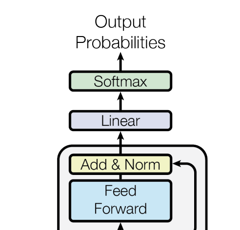
Attention is all you need

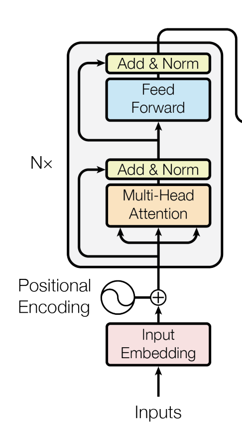
Below is one of the most snapshoted diagram in all of Machine Learning. Without this, any new blog post is incomplete. So, here it is:

Parameters and descriptions

Now comes the important stuff. What are the main parameters that the Transformers use? I describe some of them below.

• Vocab Size: All the tokens that can be part of the input sequence. Sequences are tokenized based on the vocab
• Sequence Length (S): Length of the sentence or sequence fed into the tranformer
• Embedding Size (E): Size of the embedding for each node in the sequence above

$S \times E$ dimension for one sequence ($S = d_{model}$ in the paper)

$B \times S \times E$ for a batch size of B

From paper:

To facilitate these residual connections, all sub-layers in the model, as well as the embedding layers, produce outputs of dimension $d_{model} = 512$.

• Number of Heads: Number of heads in the attention layer - output from embedding layer is split into these heads
• Head dimension: Can be calculated from embedding dimension and number of heads: embedding_size // num_heads (same as $d_k$ in the paper)

From paper:

We call our particular attention “Scaled Dot-Product Attention” (Figure 2). The input consists of queries and keys of dimension $d_k$, and values of dimension $d_v$

Scaled Dot Product Attention

• Dropout: Dropout rate after attention layer
• Feed Forward Hidden size: Hidden dimension for feed forward layer (effectively an MLP)

Encoder

Encoder Overview

One of the resources I found that illustrates the internals of Transformer architecture is Jay Alammar’s Blog Post - The Illustrated Transformer. Below is the encoder internals from the post.

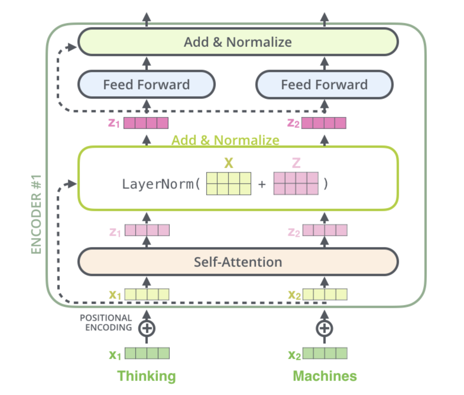
Below is the pseudo-code for how Encoder layer processes inputs and passes them from one layer to another

• Input -> Token Embedding: Embedding layer that converts tokens to embeddings
• X = Token Embedding + Position Embedding: Add position embeddings to token embeddings - this completes the input layer
• Calculate A_out = MultiHeadAttn(X): Calculate multi-head attention output
• A_out = Dropout(A_out): Apply dropout to the multi-head attention output
• L_out = LayerNorm(A_out + X): Add residual connection from input to the multi-head attention output and apply layer normalization
• F_out = FeedForwardNN(L_out): Pass the output from the multi-head attention through a feed forward network
• F_out = Dropout(F_out): Apply dropout to the feed forward network output
• out = LayerNorm(F_out + L_out): Add residual connection from the multi-head attention output to the feed forward network output and apply layer normalization

Exploration

For exploration, I will use 1984 book text. I have used this one of my previous posts as well to generate new chapters using LSTM (old times). For tokenizing, I will use the GPT2 tokenizer.

# Load the tokenizer
tokenizer = AutoTokenizer.from_pretrained('gpt2')

# Read the novel from the text file
with open('./data/1984.txt', 'r', encoding='utf-8') as file:
    novel_text = file.read()

encoded_input = tokenizer(novel_text, return_tensors='pt')
encoded_input

# output
# {'input_ids': tensor([[14126,   352,   628,  ..., 10970, 23578,   198]]), 'attention_mask': tensor([[1, 1, 1,  ..., 1, 1, 1]])}

Let’s set sequence length to be something reasonable for testing and exploration:

sequence_length = 10

For generating the inputs to the models, I use a window length of 1 to slide the sequence along to generate several sequences from our input text.

model_inputs = encoded_input["input_ids"].ravel().unfold(0, sequence_length, 1).to(torch.int32)
model_inputs

# output
# tensor([[14126,   352,   628,  ...,   257,  6016,  4692],
#        [  352,   628,   198,  ...,  6016,  4692,  1110],
#        [  628,   198,   198,  ...,  4692,  1110,   287],
#        ...,
#        [ 2739,   257,  3128,  ...,   198,   198, 10970],
#        [  257,  3128,   355,  ...,   198, 10970, 23578],
#        [ 3128,   355, 32215,  ..., 10970, 23578,   198]], dtype=torch.int32)

Let us generate a sample batch we will use for exploration.

batch_size = 4
batch = model_inputs[:batch_size, :]
batch

# output
# tensor([[14126,   352,   628,   198,   198,  1026,   373,   257,  6016,  4692],
#        [  352,   628,   198,   198,  1026,   373,   257,  6016,  4692,  1110],
#        [  628,   198,   198,  1026,   373,   257,  6016,  4692,  1110,   287],
#        [  198,   198,  1026,   373,   257,  6016,  4692,  1110,   287,  3035]],
#       dtype=torch.int32)

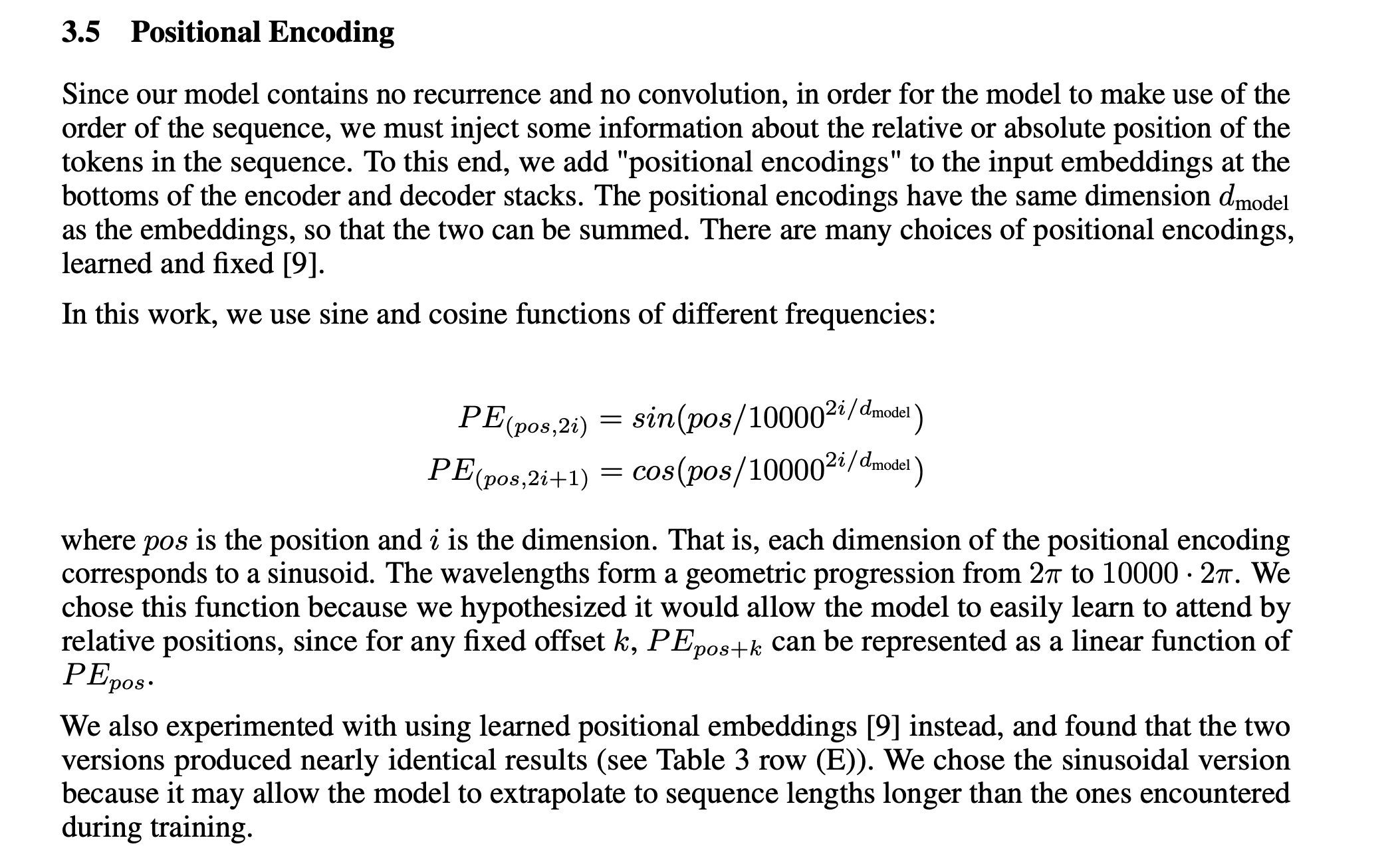
Position Encoding

Quoting from the original paper, positional encoding are just functions over the sequence and embedding dimensions.

NOTE: GPT2 onwards, positional encoding is usually added as learnable embedding instead.

Let’s generate this step by step. First, we need to generate the indices.

embedding_dimension = 6 # $d_{model}$
even_index = torch.arange(0, embedding_dimension, 2)
odd_index = torch.arange(1, embedding_dimension, 2)
print(even_index)
# tensor([0, 2, 4])

print(odd_index)
# tensor([1, 3, 5])

From here, we should be able to generate

denominator = torch.pow(10000, even_index / embedding_dimension)
print(denominator) # for odd, denominator is the same
# tensor([  1.0000,  21.5443, 464.1590])

Now, we can generate the indices along the sequence dimension.

positions = torch.arange(0, sequence_length, 1).reshape(sequence_length, 1)
print(positions)
# tensor([[0],
#         [1],
#         [2],
#         [3],
#         [4],
#         [5],
#         [6],
#         [7],
#         [8],
#         [9]])

We should have everything now to calculate the position embeddings.

even_pe = torch.sin(positions / denominator)
odd_pe = torch.cos(positions / denominator)
stacked = torch.stack([even_pe, odd_pe], dim=2)
position_embeddings = torch.flatten(stacked, start_dim=1, end_dim=2)

print(position_embeddings)
#tensor([[ 0.0000,  1.0000,  0.0000,  1.0000,  0.0000,  1.0000],
#        [ 0.8415,  0.5403,  0.0464,  0.9989,  0.0022,  1.0000],
#        [ 0.9093, -0.4161,  0.0927,  0.9957,  0.0043,  1.0000],
#        [ 0.1411, -0.9900,  0.1388,  0.9903,  0.0065,  1.0000],
#        [-0.7568, -0.6536,  0.1846,  0.9828,  0.0086,  1.0000],
#        [-0.9589,  0.2837,  0.2300,  0.9732,  0.0108,  0.9999],
#        [-0.2794,  0.9602,  0.2749,  0.9615,  0.0129,  0.9999],
#        [ 0.6570,  0.7539,  0.3192,  0.9477,  0.0151,  0.9999],
#        [ 0.9894, -0.1455,  0.3629,  0.9318,  0.0172,  0.9999],
#        [ 0.4121, -0.9111,  0.4057,  0.9140,  0.0194,  0.9998]])

Input Layer

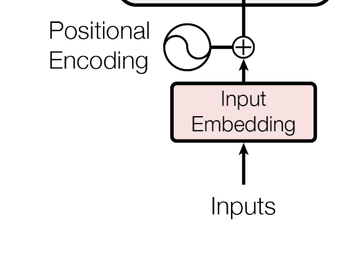
We now define the input layer i.e. the layer where sequences are converted to embeddings and then combined (added to) with position embeddings.

class InputLayer(nn.Module):
    def __init__(self, 
                 num_embeddings: int, 
                 sequence_length: int, 
                 embedding_dimension: int):
        super().__init__()
        self.sequence_length = sequence_length
        self.embedding_dimension = embedding_dimension
        self.input_embeddings = nn.Embedding(num_embeddings=num_embeddings, 
                                             embedding_dim=embedding_dimension)
        self.position_embeddings = self._init_position_embedding(sequence_length, embedding_dimension)
        print(sequence_length, embedding_dimension)

    @staticmethod
    def _init_position_embedding(sl: int, ed: int) -> torch.Tensor:
        even_index = torch.arange(0, embedding_dimension, 2)
        odd_index = torch.arange(1, embedding_dimension, 2)
        denominator = torch.pow(10000, even_index / embedding_dimension)
        even_pe = torch.sin(positions / denominator)
        odd_pe = torch.cos(positions / denominator)
        stacked = torch.stack([even_pe, odd_pe], dim=2)
        return torch.flatten(stacked, start_dim=1, end_dim=2)
        
    
    def forward(self, input: torch.Tensor) -> torch.Tensor:
        emb = self.input_embeddings(input)
        return emb + self.position_embeddings
input_layer = InputLayer(num_embeddings=len(tokenizer.get_vocab()), sequence_length=sequence_length, embedding_dimension=embedding_dimension)

We had generated a batch previously. Now we can pass the batch through the input layer to output embeddings that feed into the attention layers.

attention_input = input_layer(batch)
print(attention_input.size())
# torch.Size([4, 10, 6])

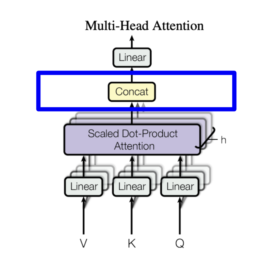
Multi Head Attention

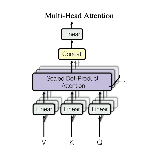
Now comes the fun part i.e. attention. We will work 2 heads (h) for demonstration purposes. head_dimension is calculated as embedding_dimension // num_heads and should be divisible by num_heads.

num_heads = 2
head_dimension = embedding_dimension // num_heads
if embedding_dimension % num_heads != 0:
    raise ValueError("embedding_dimension should be divisible by num_heads")

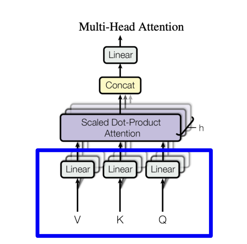
Now, we need to split the input into Q, K, and V. We can do this by passing the input through a linear layer that outputs 3 times the embedding dimension.

# split up input into Q, K, V
qkv_layer = nn.Linear(embedding_dimension, 3 * embedding_dimension)
with torch.no_grad():
    qkv_layer.weight.fill_(2)

qkv = qkv_layer(attention_input)
print(qkv.size())
# torch.Size([4, 10, 18])

What is the dimension of qkv?

It is batch_size x sequence_length x 3 * embedding_dimension

At this point, we can get to splitting of input input multiple heads i.e. multi-head attention. We have previously calculated the head dimension and number of heads.

To split, we reshape the input to batch_size x sequence_length x num_heads x 3 * head_dimension i.e. split the final dimension.

input_shape = attention_input.shape
input_shape = input_shape[:-1] + (num_heads, 3 * head_dimension)
print(input_shape)
# torch.Size([4, 10, 2, 9])

To make the attention calculation easier, we permute the dimensions to batch_size x num_heads x sequence_length x 3 * head_dimension.

Why do we permute the dimensions?

Head dimension now becomes a batch dimension. This makes it easier to calculate the attention scores on the last 2 dimensions.

Here’s the code:

qkv = qkv.reshape(*input_shape)
qkv = qkv.permute(0, 2, 1, 3)
print(qkv.size()) # batch_size, num_head, sequence_length, 3 * head_dim
# torch.Size([4, 2, 10, 9])

From the qkv output, we them back into Q, K, and V.

q, k, v = qkv.chunk(3, dim=-1)

We can calculate the attention scores with or without masking. For the encoder, we do not need masking. For the decoder, we need masking to prevent the model from looking into the future.

Below we define the masks that will be used for decode and encoder, respotively.

for masked in [True, False]:
    if masked:
        mask = torch.full((sequence_length, sequence_length),
                          -torch.inf)
        mask = torch.triu(mask, diagonal=1)
    else:
        mask = torch.zeros((sequence_length, sequence_length))
    print(mask)

tensor([[0., -inf, -inf, -inf, -inf, -inf, -inf, -inf, -inf, -inf],
        [0., 0., -inf, -inf, -inf, -inf, -inf, -inf, -inf, -inf],
        [0., 0., 0., -inf, -inf, -inf, -inf, -inf, -inf, -inf],
        [0., 0., 0., 0., -inf, -inf, -inf, -inf, -inf, -inf],
        [0., 0., 0., 0., 0., -inf, -inf, -inf, -inf, -inf],
        [0., 0., 0., 0., 0., 0., -inf, -inf, -inf, -inf],
        [0., 0., 0., 0., 0., 0., 0., -inf, -inf, -inf],
        [0., 0., 0., 0., 0., 0., 0., 0., -inf, -inf],
        [0., 0., 0., 0., 0., 0., 0., 0., 0., -inf],
        [0., 0., 0., 0., 0., 0., 0., 0., 0., 0.]])
tensor([[0., 0., 0., 0., 0., 0., 0., 0., 0., 0.],
        [0., 0., 0., 0., 0., 0., 0., 0., 0., 0.],
        [0., 0., 0., 0., 0., 0., 0., 0., 0., 0.],
        [0., 0., 0., 0., 0., 0., 0., 0., 0., 0.],
        [0., 0., 0., 0., 0., 0., 0., 0., 0., 0.],
        [0., 0., 0., 0., 0., 0., 0., 0., 0., 0.],
        [0., 0., 0., 0., 0., 0., 0., 0., 0., 0.],
        [0., 0., 0., 0., 0., 0., 0., 0., 0., 0.],
        [0., 0., 0., 0., 0., 0., 0., 0., 0., 0.],
        [0., 0., 0., 0., 0., 0., 0., 0., 0., 0.]])

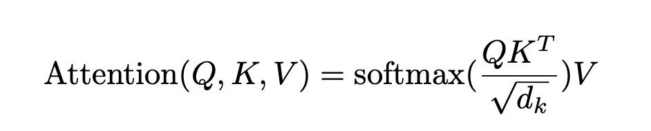
Scaled Dot Product Attention

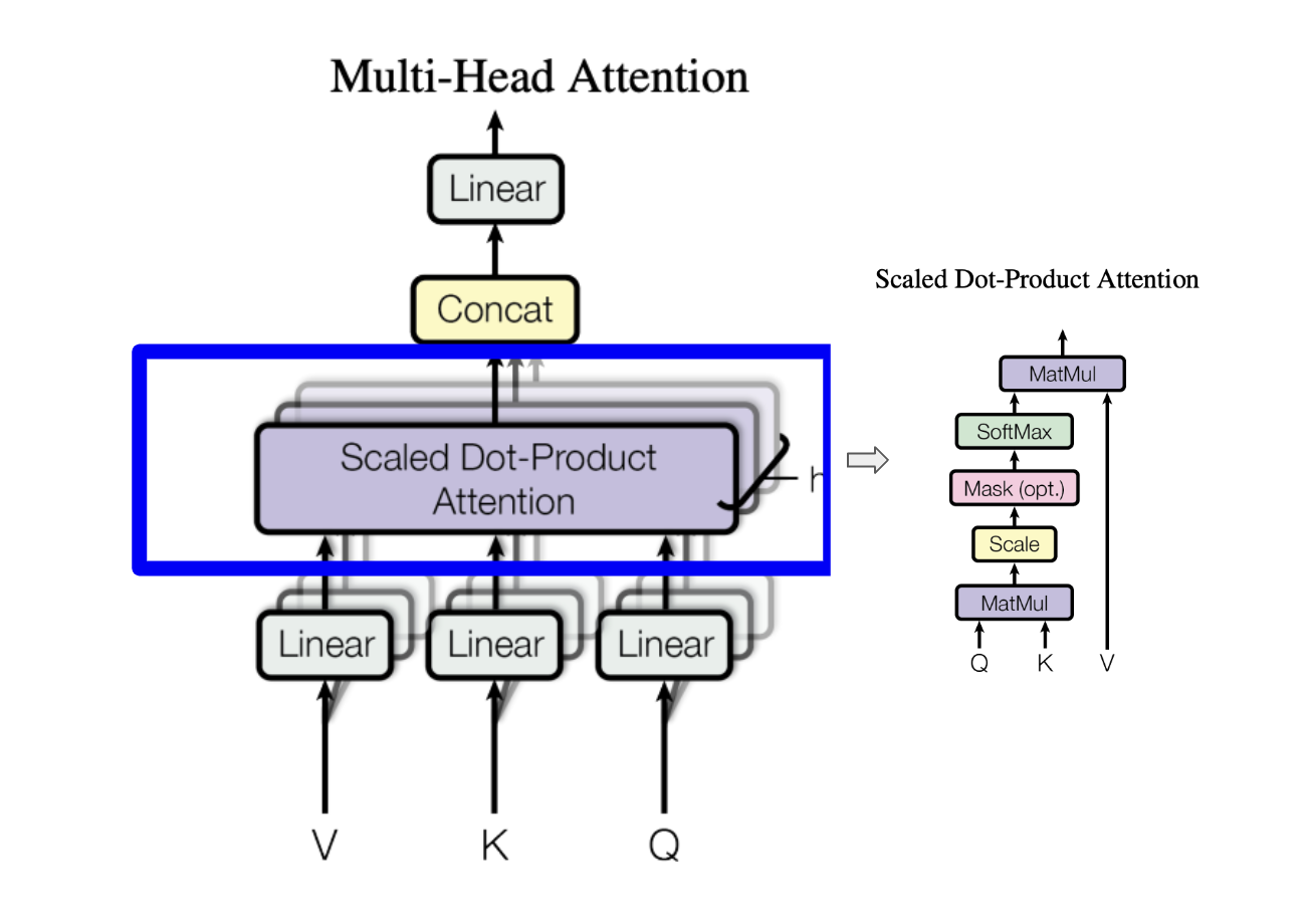
The specific flavor of attention that is commonly used now is the Scaled Dot Product Attention as described in the section above.

First, we take the query and key head blocks and do the scaled multiply

scores = torch.matmul(q, k.transpose(-2, -1)) / math.sqrt(head_dimension)

Now, we add the masks for backward looking bias (for encoder the masks are all 0 since we use both forward and backward context). After this, finally we calculate the attention scores.

scores += mask
# softmax(QK/sqrt($d_{model}$))
attention = torch.softmax(scores, dim=-1)
print(attention.size())
# torch.Size([4, 2, 10, 10])

Now, we multiply the attention scores with the value head block to get the final output.

values = torch.matmul(attention, v)
print(values.size())
torch.Size([4, 2, 10, 3])

Scaled Dot Product Attention also exists in Pytorch as torch.nn.functional.scaled_dot_product_attention.

As originally, we had changed the dimension such that the head dimension was the batch dimension, we need to change it back to the original shape. We first transpose the head and sequence dimensions and then concatenate all the head dimensions.

values = values.transpose(1, 2).contiguous()
print("After transposing the head and sequence dims", values.size())
values = values.view(*values.shape[:2], -1)
print("After concating all the head dims", values.size())

# After transposing the head and sequence dims torch.Size([4, 10, 2, 3])
# After concating all the head dims torch.Size([4, 10, 6])

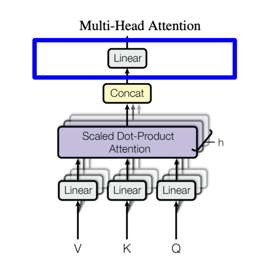
Finally, we pass the output through a linear layer to get the final output from the attention layer.

# final linear layer in the attention
attn_linear_layer = nn.Linear(embedding_dimension, embedding_dimension)
attn_out = attn_linear_layer(values)
print("output from attention has size", attn_out.size())
# output from attention has size torch.Size([4, 10, 6])

Layer Normalization

Layer Normalization (LayerNorm) in Transformer architectures normalizes inputs across features for each training instance, addressing internal covariate shift. It involves normalizing by subtracting the mean and dividing by the standard deviation, followed by an affine transformation with learnable parameters. This is done to stabilize inputs, ensuring stable and faster training.

Original transformers paper applied LayerNorm after the attention score calculation. In more recent architectures, LayerNorm (RMSNorm, etc) is applied before the attention mechanism and the feed-forward network.

Pytorch already has a LayerNorm implementation. We can use it as below:

NOTE: LayerNorm is applied after both Attention and FeedForward blocks.

# there is already a layer norm implementation in pytorch

layer_norm = nn.LayerNorm(embedding_dimension)
layer_norm_out = layer_norm(attn_out + attention_input) # attention_input is the residual connection
print(layer_norm_out.size())
# torch.Size([4, 10, 6])
print(layer_norm_out)

tensor([[-0.8153, -0.8156, -0.8156, -0.8085,  1.0473, -0.8156,  1.0442, -0.8156,
         -0.8154, -0.8156],
        [-0.8104, -0.8104, -0.8104, -0.7993, -0.8104,  0.9674, -0.8104, -0.8104,
         -0.8104, -0.8104],
        [-0.8103, -0.8102, -0.8101, -0.8104,  0.9485, -0.8101, -0.8101, -0.8104,
         -0.8104, -0.8102],
        [-0.8271, -0.8271, -0.8271,  0.9603, -0.8267, -0.8244, -0.8271, -0.8271,
         -0.8271, -0.8271]], grad_fn=<SelectBackward0>)

Let’s calculate it from scratch and we should get the same output as above.

attn_out_mean = attn_out.mean(-1, keepdim=True)
attn_out_var = torch.pow(attn_out - attn_out_mean, 2).mean(-1, keepdims=True)
attn_out_std = torch.sqrt(attn_out_var + layer_norm.eps)
ln_out = (attn_out - attn_out_mean) / attn_out_std
ln_out[:, :, 0]

tensor([[-0.8153, -0.8156, -0.8156, -0.8085,  1.0473, -0.8156,  1.0442, -0.8156,
         -0.8154, -0.8156],
        [-0.8104, -0.8104, -0.8104, -0.7993, -0.8104,  0.9674, -0.8104, -0.8104,
         -0.8104, -0.8104],
        [-0.8103, -0.8102, -0.8101, -0.8104,  0.9485, -0.8101, -0.8101, -0.8104,
         -0.8104, -0.8102],
        [-0.8271, -0.8271, -0.8271,  0.9603, -0.8267, -0.8244, -0.8271, -0.8271,
         -0.8271, -0.8271]], grad_fn=<SelectBackward0>)

Feed Forward Network

Feed forward network is a simple 2 layer MLP with ReLU activation and dropout.

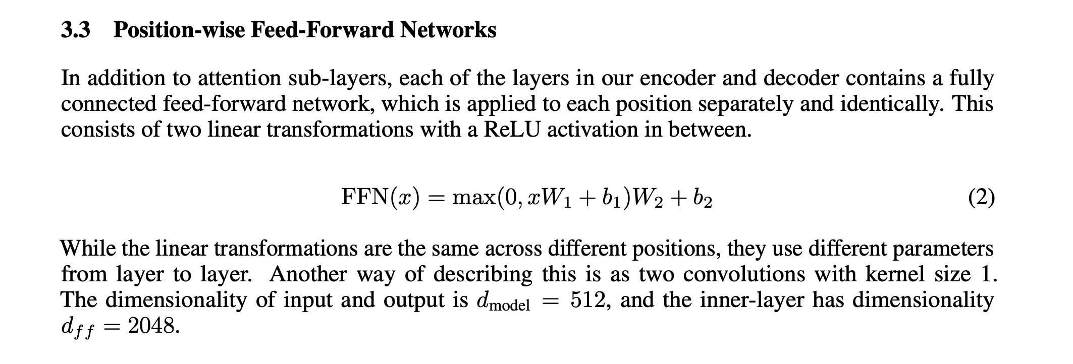
The dimensionality of input and output is \(d_{model}\) = 512, and the inner-layer has dimensionality $d_f$ = 2048.

class FeedForwardNetwork(nn.Module):
    def __init__(self, 
                 embedding_dimension: int, 
                 hidden_dimension: int, 
                 drop_prop: float):
        super().__init__()
        self.linear1 = nn.Linear(in_features=embedding_dimension, out_features=hidden_dimension)
        self.activation = nn.ReLU()
        self.dropout = nn.Dropout()
        self.linear2 = nn.Linear(in_features=hidden_dimension, out_features=embedding_dimension)

    def forward(self, x):
        return self.linear2(self.dropout(self.activation(self.linear1(x))))

Let’s test this:

ffn_hidden_dimension = 12
dropout_prob = 0.1
ffn = FeedForwardNetwork(embedding_dimension=embedding_dimension, hidden_dimension=ffn_hidden_dimension, drop_prop=dropout_prob)
ffn_out = ffn(layer_norm_out)
print(ffn_out.size())
# torch.Size([4, 10, 6])

At this point, ffn output also goes through a layer normalization

ffn_layer_norm = nn.LayerNorm(embedding_dimension)
ffn_layer_norm_out = ffn_layer_norm(ffn_out + layer_norm_out) # layer_norm_out is the residual connection
print(ffn_layer_norm_out.size())
# torch.Size([4, 10, 6])

At this point, we get the final output from the encoder layer. This in itself is a complete architecture used in encoder only networks.

Most widely known encoder only model is BERT: Bidirectional Encoder Representations from Transformers that was released by Google.

Decoder

Now we will start digging into the decoder side. For the most part, decoder part should look very similar to encoder side. Hence, we will reuse a lot of the code that we have already written.

Here’s the pseudo-code for the decoder layer:

• Input -> Sparse Embedding: Embedding layer that converts tokens to embeddings
• X = Sparse Embedding + Position Embedding (Masked): Add position embeddings to token embeddings - this completes the input layer
• Calculate A_out = MultiHeadAttn(X):: Calculate multi-head attention output (this is self-attention i.e. similar to encoder but with masking)
• A_out = Dropout(A_out): Apply dropout to the multi-head attention output
• L_out = LayerNorm(A_out + X): : Add residual connection from input to the multi-head attention output and apply layer normalization
• C_out = MultiHeadCrossAttn(L_out, encoder_out): Cross attention with encoder output
• C_out = Dropout(A_out): Apply dropout to the cross attention output
• LC_out = LayerNorm(C_out + L_out): Add residual connection to output from cross attention + dropout and apply layer normalization
• F_out = FeedForwardNN(LC_out):: Pass the output from the multi-head attention through a feed forward network (similar to encoder)
• F_out = Dropout(F_out): Apply dropout to the feed forward network output
• out = LayerNorm(F_out + LC_out): Add residual connection from the multi-head attention output to the feed forward network output and apply layer normalization

Special Tokens

Since, decoder processes inputs shifted by 1 and accounts for the start of text as being it’s own token, we need to update our tokenizer to add this “start of text” token now.

Based on the GPT2 paper, it was only trained with the endoftext token. So, we will use endoftext special token itself for the start of text token. There was a helpful discussion on Github regarding this.

Here’s an example of how we will use the <|endoftext|> token.

text = "<|endoftext|> machine learning using PyTorch"
encoded_ids = tokenizer.encode(text)
print(encoded_ids)
for id in encoded_ids:
    print(
        f"""{id:<7} = {"'" + tokenizer.convert_ids_to_tokens(id) + "":<10}'""")

[50256, 4572, 4673, 1262, 9485, 15884, 354]
50256   = '<|endoftext|>'
4572    = 'Ġmachine '
4673    = 'Ġlearning'
1262    = 'Ġusing   '
9485    = 'ĠPy      '
15884   = 'Tor      '
354     = 'ch       '

Let’s add the <|endoftext|> token to the original encoded inputs to generate the decoder input

print("encoder input: ", encoded_input["input_ids"][:, :10])
print("decoder_input: ", torch.cat(
    (torch.Tensor([[tokenizer.convert_tokens_to_ids("<|endoftext|>")]]), 
     encoded_input["input_ids"]), 
    dim=-1)[:, :10])

encoder input:  tensor([[14126,   352,   628,   198,   198,  1026,   373,   257,  6016,  4692]])
decoder_input:  tensor([[50256., 14126.,   352.,   628.,   198.,   198.,  1026.,   373.,   257.,
          6016.]])

Now, we can get a decoder input batch.

batch_size = 4

decoder_input = torch.cat((torch.Tensor([[tokenizer.convert_tokens_to_ids("<|endoftext|>")]]),  encoded_input["input_ids"]), dim=-1).to(torch.int32)
model_inputs = decoder_input.ravel().unfold(0, sequence_length, 1).to(torch.int32)
decoder_batch = model_inputs[:4, :]
print(decoder_batch)

tensor([[50256, 14126,   352,   628,   198,   198,  1026,   373,   257,  6016],
        [14126,   352,   628,   198,   198,  1026,   373,   257,  6016,  4692],
        [  352,   628,   198,   198,  1026,   373,   257,  6016,  4692,  1110],
        [  628,   198,   198,  1026,   373,   257,  6016,  4692,  1110,   287]],
       dtype=torch.int32)

Awesome, now let’s feed this input through the decoder layers

Decoder Input Layer

decoder_input_layer = InputLayer(num_embeddings=len(tokenizer.get_vocab()), sequence_length=sequence_length, embedding_dimension=embedding_dimension)
decoder_attention_input = decoder_input_layer(decoder_batch)
print("decoder attention input size:", decoder_attention_input.size())
print(decoder_attention_input[:2, :2]) # let's print a small portion of the embeddings

decoder attention input size: torch.Size([4, 10, 6])
tensor([[[-0.1335, -0.0668, -0.7628,  0.2519,  1.1015,  1.2907],
         [ 1.4312, -0.1118,  1.6050, -0.2935, -0.0866,  1.5548]],

        [[ 0.5897,  0.3479,  1.5586, -0.2924, -0.0887,  1.5548],
         [ 1.7546, -0.2418,  2.1068,  0.6056, -1.0535, -0.3810]]],
       grad_fn=<SliceBackward0>)

Decoder Self Attention Layer

Based on our exploration in encoder section, we can define a proper module for ScaledDotProductAttention and MultHeadAttention. Let’s do that first.

class ScaledDotProductAttention(nn.Module):
    def __init__(self, sequence_length: int, d_k: int, masked: bool) -> None:
        super(ScaledDotProductAttention, self).__init__()
        self.d_k = d_k
        if masked:
            mask = torch.full((sequence_length, sequence_length),
                              -torch.inf)
            self.mask = torch.triu(mask, diagonal=1)
        else:
            self.mask = torch.zeros((sequence_length, sequence_length))

    def forward(self, q: torch.Tensor, k: torch.Tensor, v: torch.Tensor):
        scores = torch.matmul(q, k.transpose(-2, -1)) / math.sqrt(self.d_k)
        scores += self.mask
        attention = F.softmax(scores, dim=-1)
        return torch.matmul(attention, v), attention

class MultiHeadAttention(nn.Module):
    def __init__(self, embedding_dimension: int, sequence_length: int,
                 num_heads: int, masked: bool = False) -> None:
        super(MultiHeadAttention, self).__init__()
        self.head_dimension = embedding_dimension // num_heads
        self.num_heads = num_heads
        self.q_linear = nn.Linear(embedding_dimension, embedding_dimension)
        self.k_linear = nn.Linear(embedding_dimension, embedding_dimension)
        self.v_linear = nn.Linear(embedding_dimension, embedding_dimension)
        self.out = nn.Linear(embedding_dimension, embedding_dimension)
        self.attention_layer = ScaledDotProductAttention(
            sequence_length=sequence_length,
            d_k=self.head_dimension,
            masked=masked
        )

    def forward(self, q: torch.Tensor, k: torch.Tensor, v: torch.Tensor):
        # q, k, v have shape (batch_size, sequence_length, embedding_dimension)
        # next we apply the linear layer and then split the output into
        # num_heads
        batch_size = q.size(0)
        # second dimension is the sequence length
        output_shape = (batch_size, -1, self.num_heads, self.head_dimension)
        # we transpose the output to
        # (batch_size, num_heads, sequence_length, head_dimension)
        # this allows us to use num_heads as a batch dimension
        q = self.q_linear(q).view(*output_shape).transpose(1, 2)
        k = self.k_linear(k).view(*output_shape).transpose(1, 2)
        v = self.v_linear(v).view(*output_shape).transpose(1, 2)
        # we apply the scaled dot product attention
        x, attention = self.attention_layer(q, k, v)
        # we transpose the output back to
        # (batch_size, sequence_length, embedding_dimension)
        x = x.transpose(1, 2).contiguous().view(
            batch_size, -1, self.head_dimension * self.num_heads)
        return self.out(x), attention

Now, we can use these to first calculate the Causal Self Attention Block.

We will combine the steps where attention output is fed into LayerNorm to get input to the cross attention block.

def calculate_causal_mha_layer(q: torch.Tensor, k: torch.Tensor, v: torch.Tensor) -> torch.Tensor:
    causal_mha = MultiHeadAttention(embedding_dimension=embedding_dimension, sequence_length=sequence_length, num_heads=num_heads, masked=True)
    scores, _ = causal_mha(q, k, v) # we ignore the attention weights
    # we add a dropout layer
    dropout = nn.Dropout(dropout_prob)
    scores = dropout(scores)
    # calculate the layer norm
    layer_norm = nn.LayerNorm(embedding_dimension)
    return layer_norm(scores + q)


causal_mha_out = calculate_causal_mha_layer(decoder_attention_input, decoder_attention_input, decoder_attention_input)
print("causal mha out size:", causal_mha_out.size())

# causal mha out size: torch.Size([4, 10, 6])

Decoder Cross Attention Layer

Now that we have fed the inputs through the self attention layer, we can calculate the Cross Attention with the encoder output.

def calculate_cross_attention_layer(self_attention_output: torch.Tensor, encoder_output: torch.Tensor) -> torch.Tensor:
    cross_attention = MultiHeadAttention(embedding_dimension=embedding_dimension, sequence_length=sequence_length, num_heads=num_heads, masked=False)
    # we replace the Q with the encoder output, K and V are the self_attention_output in the decoder
    scores, _ = cross_attention(q=encoder_output, k=self_attention_output, v=self_attention_output) # we ignore the attention weights
    # we add a dropout layer
    dropout = nn.Dropout(dropout_prob)
    scores = dropout(scores)
    # calculate the layer norm
    layer_norm = nn.LayerNorm(embedding_dimension)
    return layer_norm(scores + self_attention_output)

encoder_output = ffn_layer_norm_out
cross_attention_output = calculate_cross_attention_layer(causal_mha_out, encoder_output)
print("cross attention output size:", cross_attention_output.size())
print(cross_attention_output[:2, :2])

cross attention output size: torch.Size([4, 10, 6])
tensor([[[-0.9629, -0.7597, -1.2258,  0.8206,  1.2307,  0.8972],
         [ 0.4771, -1.0049,  1.6433, -1.0474, -0.7278,  0.6597]],

        [[-0.9022,  0.1326,  1.3445, -1.3122, -0.4581,  1.1954],
         [ 0.5531, -0.0851,  1.6785,  0.2169, -1.0609, -1.3026]]],
       grad_fn=<SliceBackward0>)

Decoder Feed Forward Layer

Now, we can calculate the feed forward layer just like the encoder part of the network.

def calculate_ffn_layer(cross_attention_output: torch.Tensor) -> torch.Tensor:
    ffn = FeedForwardNetwork(embedding_dimension=embedding_dimension, hidden_dimension=ffn_hidden_dimension, drop_prop=dropout_prob)
    ffn_out = ffn(cross_attention_output)
    # no dropout since it is already applied in the FeedForwardNetwork
    ffn_layer_norm = nn.LayerNorm(embedding_dimension)
    return ffn_layer_norm(ffn_out + cross_attention_output) # cross_attention_output is the residual connection

ffn_output = calculate_ffn_layer(cross_attention_output)
print("ffn output size:", ffn_output.size())
print(ffn_output[:2, :2])

ffn output size: torch.Size([4, 10, 6])
tensor([[[-0.8360, -0.9143, -1.1446,  0.8524,  1.4350,  0.6075],
         [ 0.7893, -0.9337,  1.4718, -1.2387, -0.6771,  0.5883]],

        [[-0.2053,  0.2958,  1.1531, -1.7495, -0.5692,  1.0750],
         [ 0.6976, -0.0073,  1.5595,  0.2070, -1.1275, -1.3293]]],
       grad_fn=<SliceBackward0>)

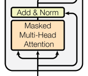
Output Probabilities

Final layer of the network calculates the probabilities for the output tokens from the network. In this layer, we pass the normalized output from FeedForward layer to Linear + Softmax.

def calculate_output_probabilities(ffn_output: torch.Tensor) -> torch.Tensor:
    # output dimension for linear layer is the vocab size
    output_linear = nn.Linear(embedding_dimension, len(tokenizer.get_vocab())) 
    return F.softmax(output_linear(ffn_output), dim=-1) # final output probabilities

output_probabilities = calculate_output_probabilities(ffn_output)
print("output probabilities size:", output_probabilities.size())

# output probabilities size: torch.Size([4, 10, 50257])

We finally have the seq2seq probabilities. We can now calculate the loss and backpropagate to train the network.

We only tested our transformer implementation with a single layer of attention. In practice, transformers have multiple layers of attention. We can stack multiple layers of the encoder and decoder to get better performance. Original transformer paper used 6 layers of attention in both encoder and decoder.

Decoder Summary

In the decoder section, we have described the different layers and operations involved in the decoder of a transformer neural network. We have discussed the self-attention layer, cross-attention layer, feed-forward layer, and the output probabilities layer. We have also provided code examples and explanations for each layer.

• The self-attention layer calculates the causal attention weights for each token in the input sequence based on its relationship with other tokens.
• The cross-attention layer performs attention over the encoder output to incorporate information from the input sequence.
• The feed-forward layer applies a non-linear transformation to the output of the cross-attention layer.
• Finally, the output probabilities layer calculates the probabilities for each token in the vocabulary.

The decoder plays a crucial role in tasks such as language translation, text generation, and sequence-to-sequence modeling.

What are the top decoder only models?

Most of the well known models are decoder only models:

• GPT
• LLAMA
• Gemini
• List goes on…

Summary

We have discussed and implemented both the encoder and decoder parts of the transformers architecture from scratch. We have analyzed how the input tokens flow through the original transformers architecture and explained the different layers and operations involved in each part.

For the encoder, we have described the self-attention layer and feed-forward layer. We have provided code examples and explanations for each layer, including the calculation of attention weights, layer normalization, etc.

Similarly, for the decoder, we have discussed the causal self-attention layer, cross-attention layer, feed-forward layer, and the output probabilities layer. We have explained how the decoder incorporates information from the encoder output and generates output probabilities based on the input sequence.

This was generally a very fruitful exercise for me. This serves as a foundational exercise to understand all major transformer models.

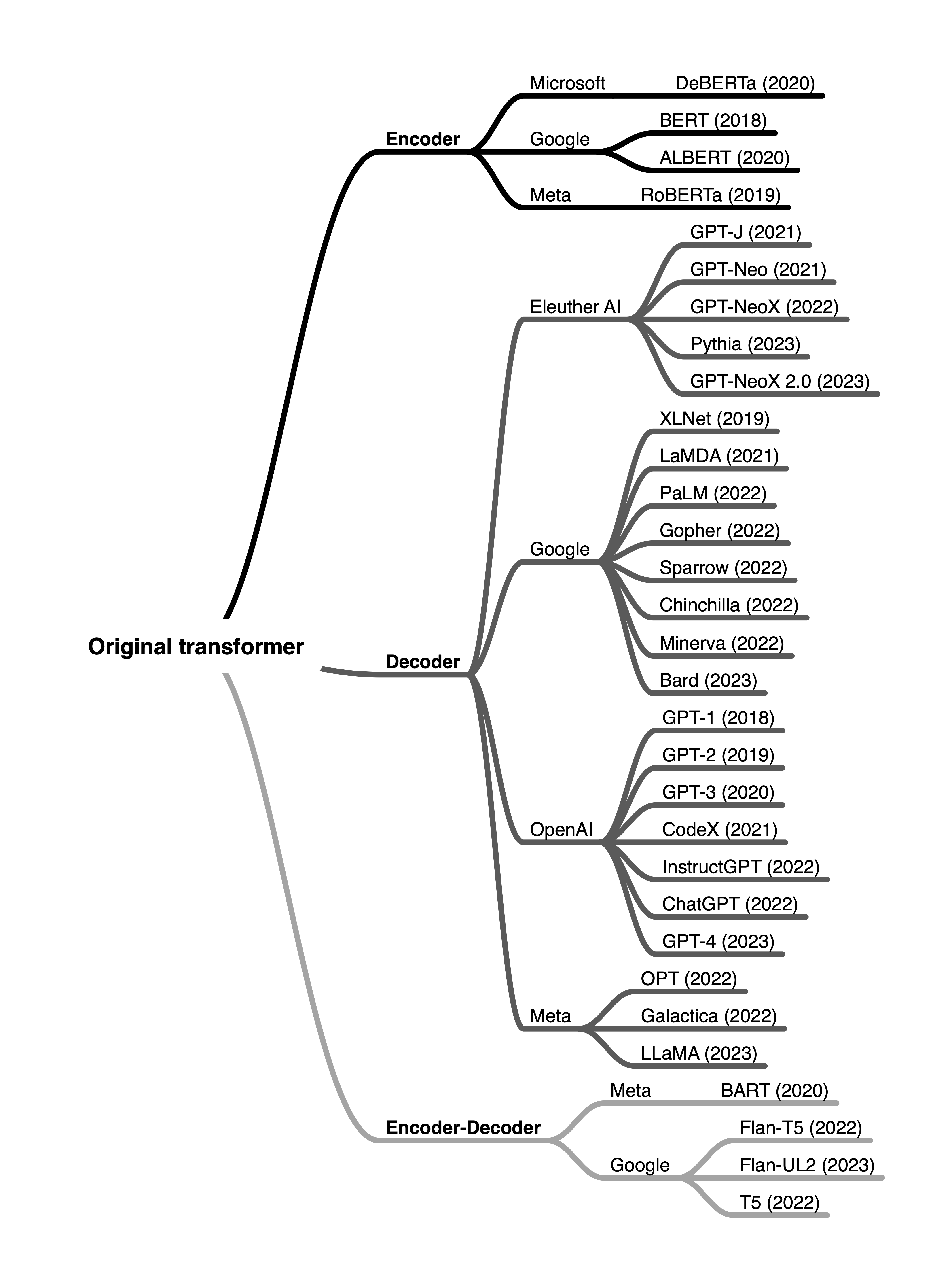
To finish up, here is a really cool graphic that shows a list of major transformers based models from Sebastian Raschka’s substacl post - Understanding Encoder And Decoder LLMs. Once you understand the original transformers architecture, you can easily understand the evolution of transformers-based models and their architectures.

Github

The code for this post is available on Github

Sources

• Attention is all you need
• Layer Normalization
• Pytorch LayerNorm
• BERT: Bidirectional Encoder Representations from Transformers
• GPT2 paper
• The Illustrated Transformer