Regularization in Linear Models

Least squares estimates are often not very satisfactory due to their poor out-of-sample performance, especially when the model is overly complex with a lot of features. We can attribute this to low bias and large variance in least squares estimates. Additionally, when we have a lot of features in our model, it is harder to explain the features with the strongest effect or what we call the Big Picture. Hence, we might want to choose fewer features in order to trade a worse in-sample variance for a better out-of-sample prediction.

Regularization is a method to shrink or drop coefficients/parameters from a model by imposing a penalty on their size. It is also referred to as the Shrinkage Method. In this post, I will discuss two of the most common regularization techniques - Ridge and Lasso regularization.

Setup

For starters, we will use the Prostate Cancer dataset from the Elements of Statistical Learning book. If you want more information about the dataset, it’s available in Chapter 1 of the book or here and the dataset is available here

If you want to follow along with some code, I have put a Jupyter Notebook on Github.

import numpy as np
import pandas as pd

import matplotlib as mpl
import matplotlib.pyplot as plt
import seaborn as sns

from logorama import logger

from bokeh.io import output_notebook, curdoc
from bokeh.plotting import figure, show
from bokeh.themes import Theme
from bokeh.embed import components
from bokeh.models import Range1d
from bokeh.palettes import Spectral10

import scipy.optimize as so

%matplotlib inline

plot_theme = Theme("./theme.yml")
output_notebook()

sns.set_style(style="dark")

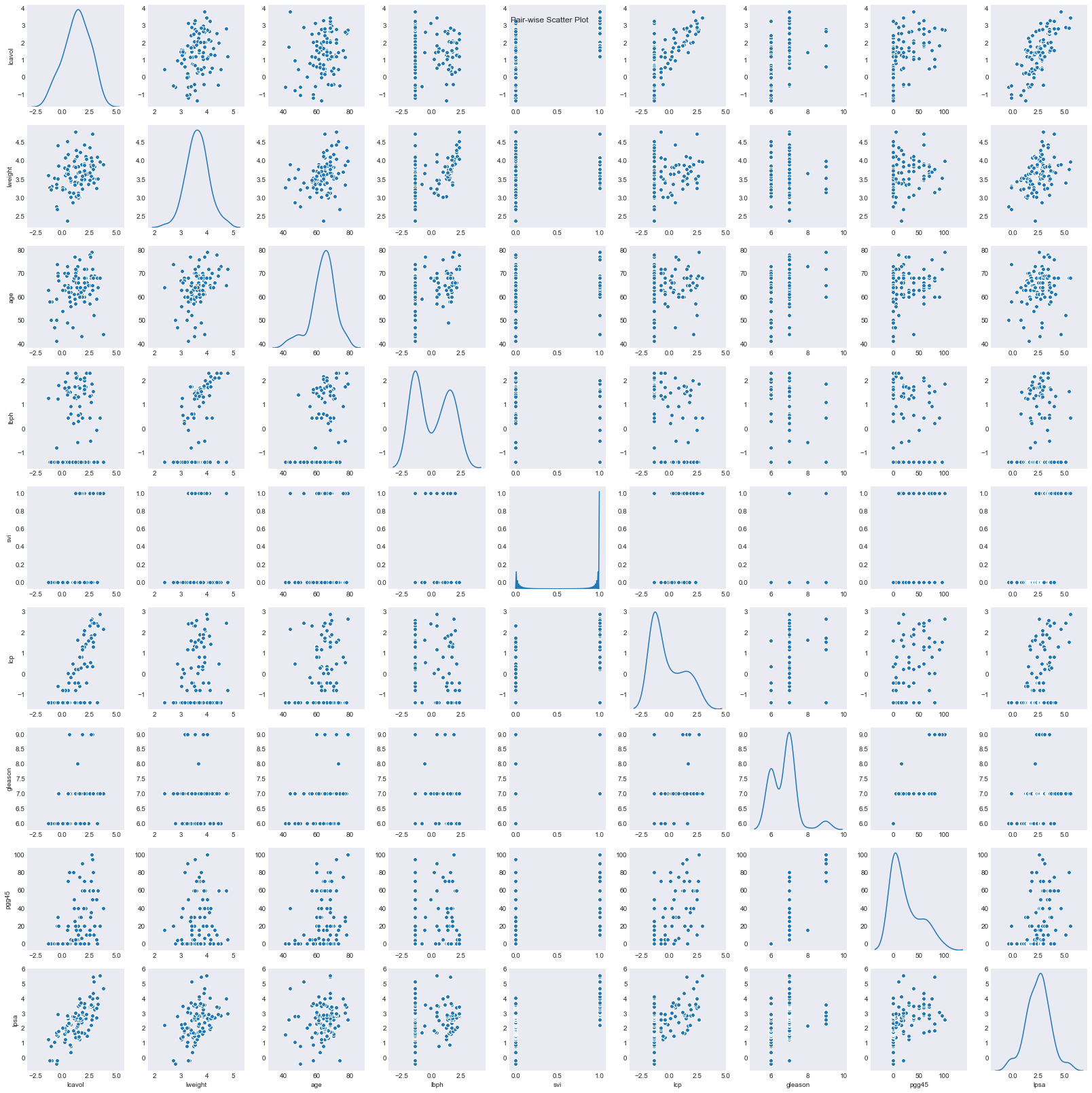
Let’s load the data and plot the pair-wise scatter plot for it.

prostate_data = pd.read_csv("https://web.stanford.edu/~hastie/ElemStatLearn/datasets/prostate.data", 
                            sep="\t", index_col=0)
train_idx = prostate_data["train"] == "T"
prostate_data.drop(columns="train", inplace=True)

fp = sns.pairplot(prostate_data, diag_kind="kde")
fp.fig.suptitle("Pair-wise Scatter Plot")
plt.show()

We will need the L2-Norm for the Linear Least Squares model, so let’s implement that.

def norm(betas, x_train, y_train):
    return np.linalg.norm(y_train - np.mean(y_train) - x_train.dot(betas))

About the dataset

The original data comes from a study by Stamey et. al. [1989], where they examined the relationship between the level of prostate-specific antigen and number of clinical measures in men who were about to receive a radical prostatectomy. Features in model are:

• log cancer volume (lcavol)
• log prostate weight (lweight )
• age (age )
• log of the amount of benign prostatic hyperplasia (lbph)
• seminal vesicle invasion (svi)
• log of capsular penetration (lcp)
• Gleason score (gleason)
• Percent of Gleason scores 4 or 5 (pgg45)

The response variable is:

• log of prostate-specific antigen (lpsa)

Simple Linear Fit

Before we jump to Ridge and Lasso regression, let’s fit a least squares model to the data and get corresponding standard error and z-score estimates for each coefficient.

We know that the linear regression fit is given by:

\begin{equation} \hat y = \mathbf{X} \beta = \mathbf{X} (\mathbf{X^\intercal} \mathbf{X})^{-1} \mathbf{X^\intercal} y \end{equation}

The variance-covariance matrix for least squares parameters is given by

\begin{equation} Var(\hat \beta) = (\mathbf{X^\intercal} \mathbf{X})^{-1} \sigma^2 \end{equation}

where $\sigma$ is the population standard deviation of $y_i$. We can estimate $\sigma^{2}$ by:

\begin{equation} \hat \sigma^2 = \dfrac{1}{N - p -1} \sum\limits_{i=1}^N (y_i - \hat y_i)^2 \end{equation}

Finally, we can calculate the z-score as:

\begin{equation} Z_{\beta_i} = \dfrac{\hat \beta_i - 0}{\hat \sigma_{\beta_i}} \end{equation}

y_data = prostate_data["lpsa"]

x_data = prostate_data.drop(columns="lpsa")
x_data = (x_data - x_data.mean()) / x_data.std() # Standardize

x_train = x_data.loc[train_idx]
x_train = np.hstack([np.ones((len(x_train), 1)), x_train.values.copy()])
y_train = y_data.loc[train_idx]

betas = np.linalg.inv(x_train.T.dot(x_train)).dot(x_train.T).dot(y_train)

y_train_hat = x_train.dot(betas) 

dof = len(x_train) - len(betas)

mse = np.sum((y_train_hat - y_train) ** 2) / dof

betas_cov = np.linalg.inv(x_train.T.dot(x_train)) * mse
betas_se = np.sqrt(betas_cov.diagonal())
betas_z = (betas - 0) / betas_se

betas_estimate_table = pd.DataFrame({"Beta": betas, "SE": betas_se, "Z-Score": betas_z}, 
                                    index=np.append(["intercept"], x_data.columns))

logger.info(f"Degrees of Freedom: {dof}")
logger.info(f"MSE: {np.round(mse, 4)}")
logger.info(f"Beta Errors:\n{betas_estimate_table}")

2018-09-08 16:09:32.860426 - [INFO] - {root:<module>:12} - Degrees of Freedom: 58
2018-09-08 16:09:32.865155 - [INFO] - {root:<module>:13} - MSE: 0.5074
2018-09-08 16:09:32.872027 - [INFO] - {root:<module>:14} - Beta Errors:
               Beta        SE    Z-Score
intercept  2.464933  0.089315  27.598203
lcavol     0.679528  0.126629   5.366290
lweight    0.263053  0.095628   2.750789
age       -0.141465  0.101342  -1.395909
lbph       0.210147  0.102219   2.055846
svi        0.305201  0.123600   2.469255
lcp       -0.288493  0.154529  -1.866913
gleason   -0.021305  0.145247  -0.146681
pgg45      0.266956  0.153614   1.737840

At a 95% confidence level, z-score greater/less than value of $\pm1.96$ is significant.

Out of the 9 features, 4 (age, lcp, gleason, pgg45) are not significant in our current model

Let’s calculate the MSE for out-of-sample/test data

x_test = x_data.loc[~train_idx]
x_test = np.hstack([np.ones((len(x_test), 1)), x_test.values.copy()])
y_test = y_data.loc[~train_idx]

y_test_hat = x_test.dot(betas) 


dof_test = len(x_test) - len(betas)
mse = np.sum((y_test_hat - y_test) ** 2) / dof_test

logger.info(f"MSE: {np.round(mse, 4)}")

2018-09-08 16:09:33.139871 - [INFO] - {root:<module>:11} - MSE: 0.7447

We can see that the variance is much higher for the out-of-sample data, as expected in case of an over-fit least squares model.

Next, let’s discuss how we can use regularization to help with this model.

Ridge Regression

Ridge regression imposes an $L_2$ norm based penalty on the sizes of coefficients given by $\beta^{\intercal} \beta$. We also introduce a complexity parameter $\lambda >= 0$ that controls the amount of shrinkage. Hence, the total shrinkage is given by $\lambda \beta^{\intercal} \beta$.

As the value of $\lambda$ gets larger, we get higher shrinkage

Our new regression coefficients are given by:

\begin{equation} \hat \beta^{ridge} = \mathbf{argmin}_{\beta} \Bigg \{ \sum _{i = 1}^N (y_i - \beta_0 - \sum _{j = 1}^p x _{ij} \beta_j )^2 + \lambda \sum _{j = 1}^p \beta _j^2 \Bigg \} \end{equation}

Inputs need to be standardized to bring Ridge coefficients to equivalent scale

Notice that $\beta_0$ is left out of the penalty term since that will make the intercept depend on origin of $Y$. In other words, if we add a constant c to all $y_i$, our intercept should not change. However, if we do include $\beta_0$ in the penalty term, the intercept will change.

Therefore, we need to re-parameterize the model such that effective $y_i$ are given by $y_i - \bar y$, where $\bar y$ is given by $\dfrac{\sum _i^N y_i}{N}$. After re-parameterization, $X$ has $p$ columns instead of $p+1$ and no constant term. Now, we can rewrite our Ridge coefficients in matrix form as:

\begin{equation} \hat \beta^{ridge} = (\mathbf{X}^\intercal \mathbf{X} + \lambda \mathbf{I})^{-1}\mathbf{X}^\intercal y \end{equation}

Next, let’s analyze the effect of $\lambda$ on shrinkage of Ridge regression coefficients. It’s easy to notice to that $\lambda = 0$ should just lead to least squares coefficients.

ridge_coeffs = np.append([0], np.logspace(0, 5.0, 21))
x_train = x_data.loc[train_idx].values.copy()
y_train = y_data.loc[train_idx].copy()
y_train = y_train - np.mean(y_train)

betas_ridge = {}
for lambdaa in ridge_coeffs:
    betas = np.linalg.inv(x_train.T.dot(x_train) + 
                          lambdaa * np.identity(len(x_train[0]))).dot(x_train.T).dot(y_train)
    betas_ridge[lambdaa] = pd.Series(betas, index=x_data.columns)
betas_ridge = pd.DataFrame(betas_ridge).T

p = figure(plot_width=800, plot_height=600)

for col, color in zip(x_data.columns, Spectral10):
    p.line(x=np.log10(betas_ridge.index.values), y=betas_ridge[col].values, legend=col, color=color)
    p.circle(x=np.log10(betas_ridge.index.values), y=betas_ridge[col].values, legend=col, color=color)
    
    
p.title.text = "Coefficient Shrinkage in Ridge Regression (\u03B2 vs log\u2081\u2080(\u03BB))"
p.xaxis.axis_label = "log\u2081\u2080(\u03BB)"
p.yaxis.axis_label = "Coefficient"
p.legend.location = "top_right"

curdoc().clear()
doc = curdoc()
doc.theme = plot_theme
doc.add_root(p)
show(p)

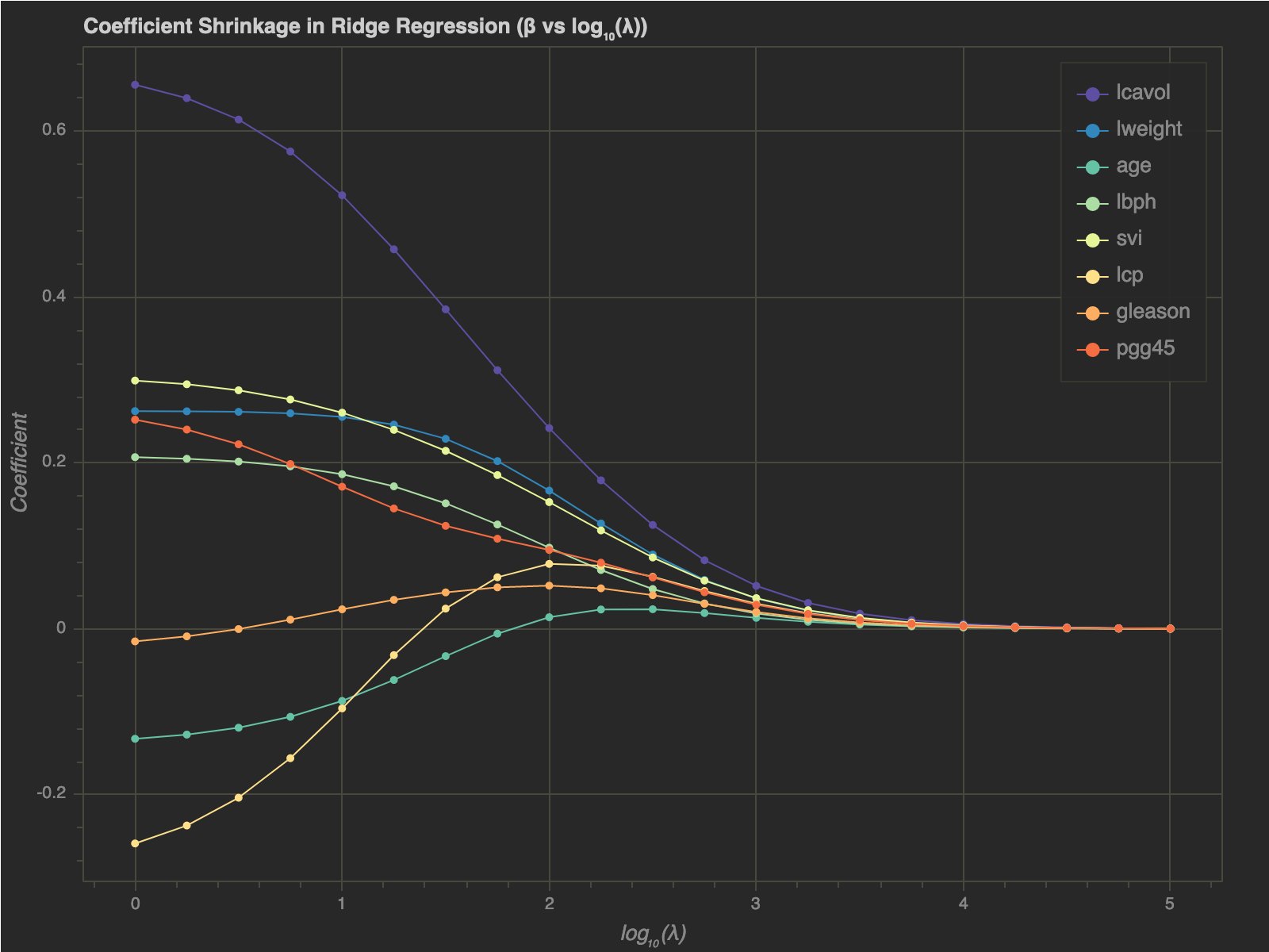
• As $\lambda$ increases, coefficients’ magnitudes get smaller
• We can see that at large values of $\lambda$, all coefficients approach $0$

One interesting thing to note is that the gradient of $|| \beta ||^2_2$ is $2 \beta$. The gradient gets smaller and smaller as $\beta$ gets closer to $\mathbf{0}$. Hence, $\beta$ asymptotically approaches $\mathbf{0}$.

Alternate Formulation

We can formulate the Ridge regression solution alternatively as:

\begin{equation} \hat \beta^{ridge} = \mathbf{argmin}_{\beta} \Bigg \{ \sum _{i = 1}^N (y_i - \beta_0 - \sum _{j = 1}^p x _{ij} \beta_j )^2 \Bigg \} \hspace{1cm} s.t. \sum _{j = 1}^p \beta _j^2 <= t \end{equation}

where there is a one-to-one correspondence betwee $\lambda$ and $t$.

If we scale $t$, such that we divide it by $\sqrt{ \sum_{j = 1}^p \beta_{ls(j)}^2}$, or ($|| \beta_{ls} ||_2$), we get a shrinkage factor, which is in the domain $[0, 1]$. Notice that I haven’t used the squared norm.. I will discuss later why I made that decision.

Let’s plot our Ridge coefficients against the shrinkage factor $\dfrac{t}{|| \beta ||_2}$:

ols_beta_norm = np.linalg.norm(betas_estimate_table.Beta.values[1:])

ridge_coeffs = np.linspace(0, ols_beta_norm, 21)
x_train = x_data.loc[train_idx].values.copy()
y_train = y_data.loc[train_idx].copy()
y_train = y_train - np.mean(y_train)

def fit_ridge(t, x_train, y_train):
    return so.minimize(
        fun=norm, x0=np.zeros(len(x_train[0])),
        constraints={
            "type": "ineq",
            "fun": lambda x: t - np.linalg.norm(x)
        },
        args=(x_train, y_train)
    )

betas_ridge = {}

for t in ridge_coeffs:
    result = fit_ridge(t, x_train=x_train, y_train=y_train)
    shrink_coeff = t / ols_beta_norm
    betas_ridge[shrink_coeff] = pd.Series(result.x, index=x_data.columns)

betas_ridge = pd.DataFrame(betas_ridge).T
betas_ridge.sort_index(inplace=True)

p = figure(plot_width=800, plot_height=600)

for col, color in zip(x_data.columns, Spectral10):
    p.line(x=betas_ridge.index, y=betas_ridge[col].values, legend=col, color=color)
    p.circle(x=betas_ridge.index, y=betas_ridge[col].values, legend=col, color=color)
    
    
p.title.text = "Coefficient Shrinkage in Ridge Regression"
p.xaxis.axis_label = "Shrinkage Factor: t / ||\u03B2||\u2082"
p.yaxis.axis_label = "Coefficient"
p.legend.location = "top_left"

curdoc().clear()
doc = curdoc()
doc.theme = plot_theme
doc.add_root(p)
show(p)

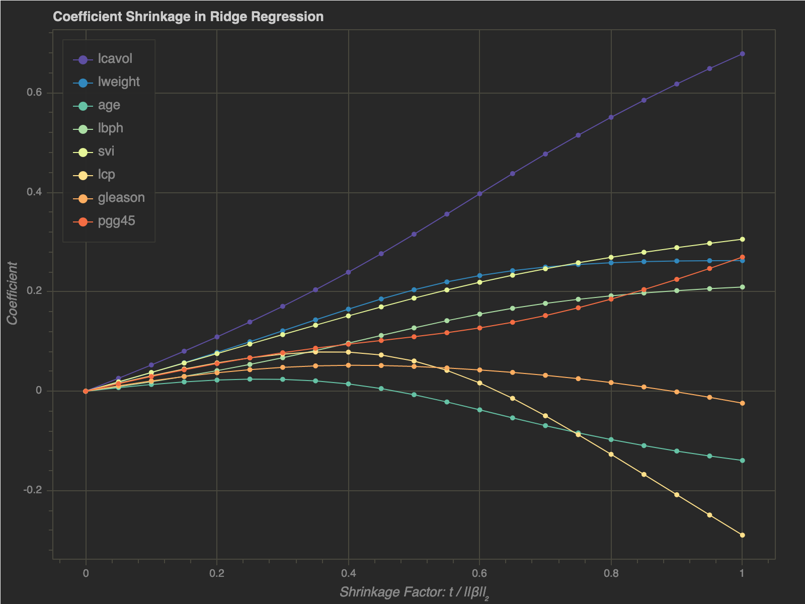
• As we can see, $t$ determines how large the coefficients can get
• If $t$ is closer to $0$, none of the betas can get too large
• On the other hand, as $t \rightarrow 1$, the coefficients get closer to the least squares coefficients

Lasso Regression

Lasso regression imposes an $L_1$ penalty to the regression coefficient compared to the $L_2$ penalty in case of Ridge. Hence, the coefficient formulation changes slightly to:

\begin{equation} \hat \beta^{lasso} = \mathbf{argmin}_{\beta} \Bigg \{ \sum _{i = 1}^N (y_i - \beta_0 - \sum _{j = 1}^p x _{ij} \beta_j )^2 + \lambda \sum _{j = 1}^p |\beta _j| \Bigg \} \end{equation}

or alternatively:

\begin{equation} \hat \beta^{lasso} = \mathbf{argmin}_{\beta} \Bigg \{ \sum _{i = 1}^N (y_i - \beta_0 - \sum _{j = 1}^p x _{ij} \beta_j )^2 \Bigg \} \hspace{1cm} s.t. \sum _{j = 1}^p |\beta _j| <= t \end{equation}

Let’s look at the shrinkage of coefficients for a range of $\lambda’s$:

lasso_coeffs = np.linspace(0, 10, 21)
x_train = x_data.loc[train_idx].values.copy()
y_train = y_data.loc[train_idx].copy()
y_train = y_train - np.mean(y_train)

def modified_norm(betas, x_train, y_train, coeff):
    return norm(betas=betas, x_train=x_train, 
                y_train=y_train) + coeff * np.sum(np.abs(betas))
    
def fit_lasso(lambdaa, x_train, y_train):
    return so.minimize(
        fun=modified_norm, x0=np.zeros(len(x_train[0])),
        args=(x_train, y_train, lambdaa)
    )

betas_lasso = {}

for lambdaa in lasso_coeffs:
    result = fit_lasso(lambdaa, x_train=x_train, y_train=y_train)
    betas_lasso[lambdaa] = pd.Series(result.x, index=x_data.columns)
    
betas_lasso = pd.DataFrame(betas_lasso).T
betas_lasso.sort_index(inplace=True)

p = figure(plot_width=800, plot_height=600)

for col, color in zip(x_data.columns, Spectral10):
    p.line(x=betas_lasso.index, y=betas_lasso[col].values, legend=col, color=color)
    p.circle(x=betas_lasso.index, y=betas_lasso[col].values, legend=col, color=color)
    
    
p.title.text = "Coefficient Shrinkage in Lasso Regression"
p.xaxis.axis_label = "\u03BB"
p.yaxis.axis_label = "Coefficient"
p.legend.location = "top_right"

curdoc().clear()
doc = curdoc()
doc.theme = plot_theme
doc.add_root(p)
show(p)

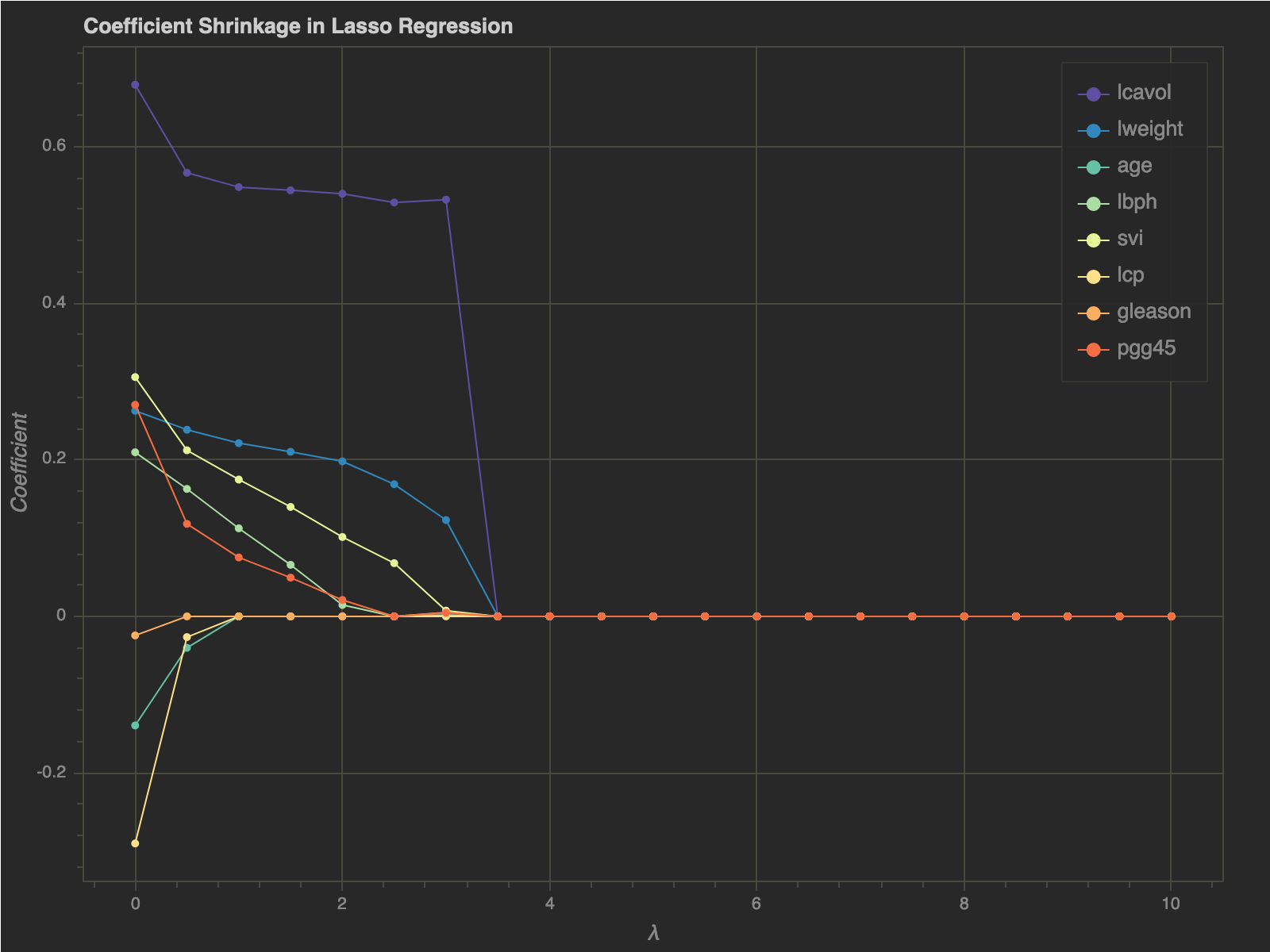
• Making $t$ sufficiently small will automatically make certain coefficients $0$
• If $t$ is chosen larger than $\sum _{j = 1}^p |\beta_j|$ (sum of absolute values of least square coefficients) Lasso coefficients are equal to least square coefficients

Again, similar to Ridge, if we scale $t$, such that we divide it by $\sum_{j = 1}^p | \beta_{ls(j)} | $, or ($|| \beta_{ls} ||_1$), we get a shrinkage factor, which is in the domain $[0, 1]$.

I used the $L_2$ norm directly instead of squaring it earlier to scale Ridge and Lasso shrinkage factors equally

Let’s plot the Lasso coefficients $w.r.t.$ the shrinkage factor:

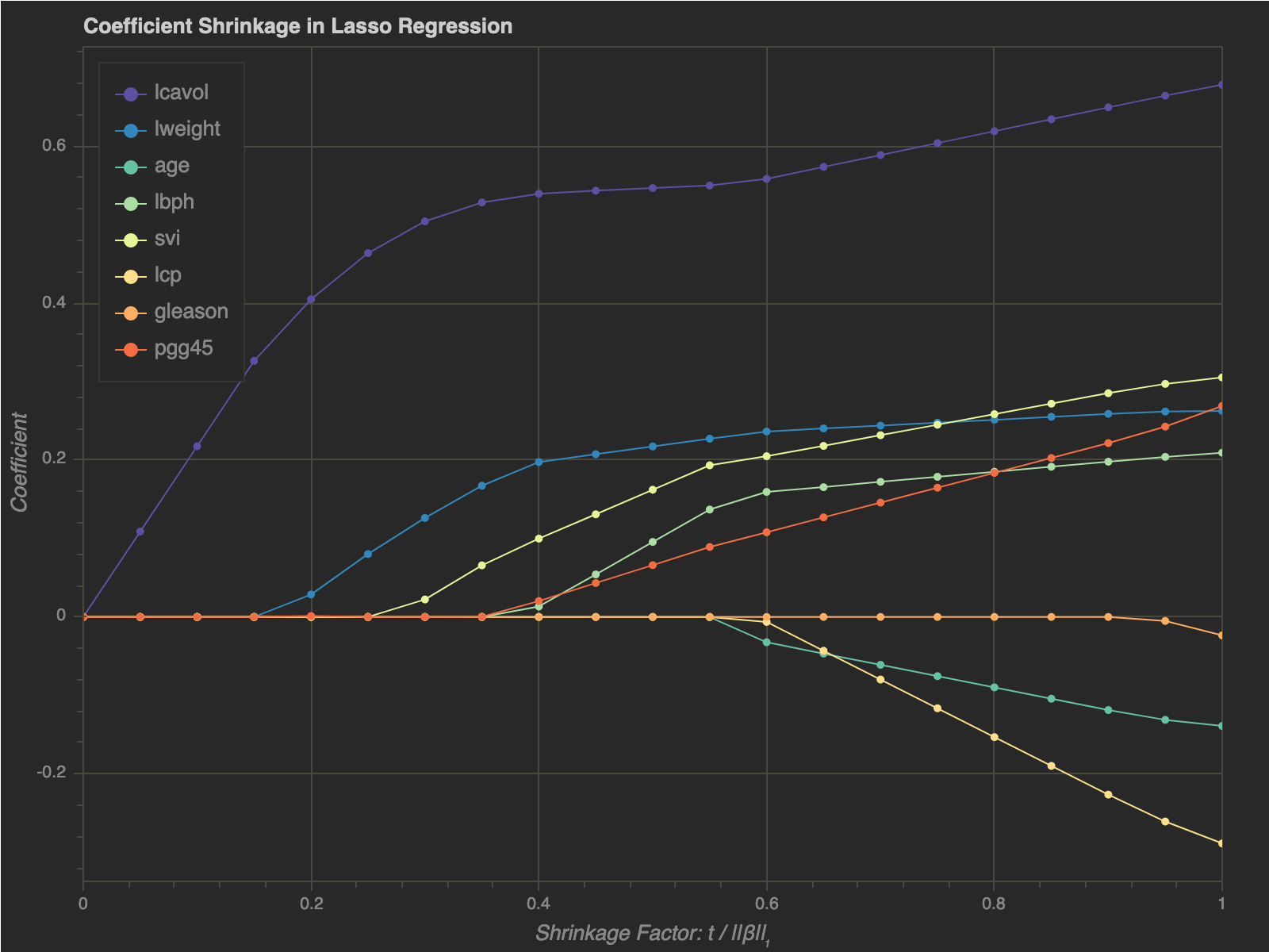
We can see that as $t$ gets sufficiently small, the coefficients start dropping out of the model. Hence, Lasso regression can be used for feature selection

Final Words

In this post, I discussed how to use regularization in the case of linear models and specifically explored Ridge and Lasso techniques. I also discussed how Ridge proportionally shrinks the least squares coefficients versus Lasso that shrinks each coefficients by a constant factor i.e. $\lambda$. Finally, we also saw how Lasso can be used for feature selection/drop-out in a linear model.

Sources

1. Elements of Statistical Learning - Chapter 3
2. Stanford STATS 305