Local Linear Regression

I previously wrote a post about Kernel Smoothing and how it can be used to fit a non-linear function non-parametrically. In this post, I will extend on that idea and try to mitigate the disadvantages of kernel smoothing using Local Linear Regression.

Setup

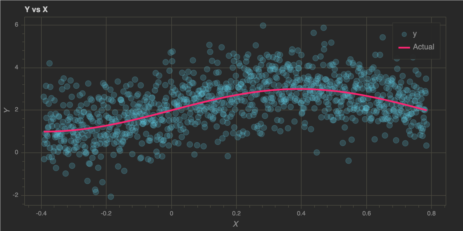
I generated some data in my previous post and I will reuse the same data for this post. The data was generated from the function $\mathbf{y = f(x) = sin(4x) + 2}$ with some Gaussian noise and here’s how it looks:

Local Linear Regression

As I mentioned in the previous article, in kernel smoothing out-of-sample predictions on the edges and in sparse regions can have significant errors and bias. In Local Linear Regression, we try to reduce this bias to first order, by fitting straight lines instead of local constants.

Local linear regression solves a weighted least squares problem at each out-of-sample point $x_0$, given by:

\begin{equation} \mathbf{\min\limits_{\alpha(x_0), \beta(x_0)} \sum\limits_{i=1}^N} K_\lambda(x_0, x_i) ( y_i - \alpha(x_0) - \beta(x_0) x_i )^2 \end{equation}

which gives us $\hat \alpha(x_0)$ and $\hat \beta(x_0)$. The estimate $\hat y_0$ is then given by:

\begin{equation} \mathbf{\hat y_0 = \hat \alpha(x_0) + \hat \beta(x_0) x_0} \end{equation}

NOTE: Even though we fit an entire linear model, we only use it to fit a single point $x_0$

Let’s formulate the matrix expression to calculate $\hat y_0$ and then implement it in Python.

Let,

• $b(x)^T$ be a 2-d vector given by: $b(x)^T = (1, x_0)$
• $\mathbf{B}$ be a $N \times 2$ matrix with the $i^{th}$ row $b(x)^T$
• $\mathbf{W(x_0)}$ be $N \times N$ diagonal matrix with $i^{th}$ diagonal element $K_\lambda(x_0, x_i)$

Then,

\begin{equation} \mathbf{\hat y_0} = b(x_0)^\intercal (\mathbf{B}^\intercal\mathbf{W}\mathbf{B})^{-1} \mathbf{B}^\intercal \mathbf{W(x_0)} \mathbf{y} \end{equation}

The final estimate $\hat y_0$ is still linear in $y_i’s$ since the weights do not depend on $y$ at all

In other words, $b(x_0)^\intercal (\mathbf{B}^\intercal\mathbf{W}\mathbf{B})^{-1} \mathbf{B}^\intercal \mathbf{W(x_0)}$ is a linear operator on $y$ and is independent of $y$

def predict(x_test, x_train, y_train, h):
    if len(x_train) != len(y_train):
        raise ValueError("X and Y Should have same length")
    B = np.array([np.ones(len(x_train)), x_train]).T
    y_hat = []
    for x0 in x_test:
        W = np.diag(gaussian_kernel(x_train , x0, h))
        y_hat.append(np.array([1, x0]).T.dot(
            np.linalg.inv(B.T.dot(W).dot(B))).dot(
            B.T).dot(W).dot(y_train))
    
    return np.array(y_hat)

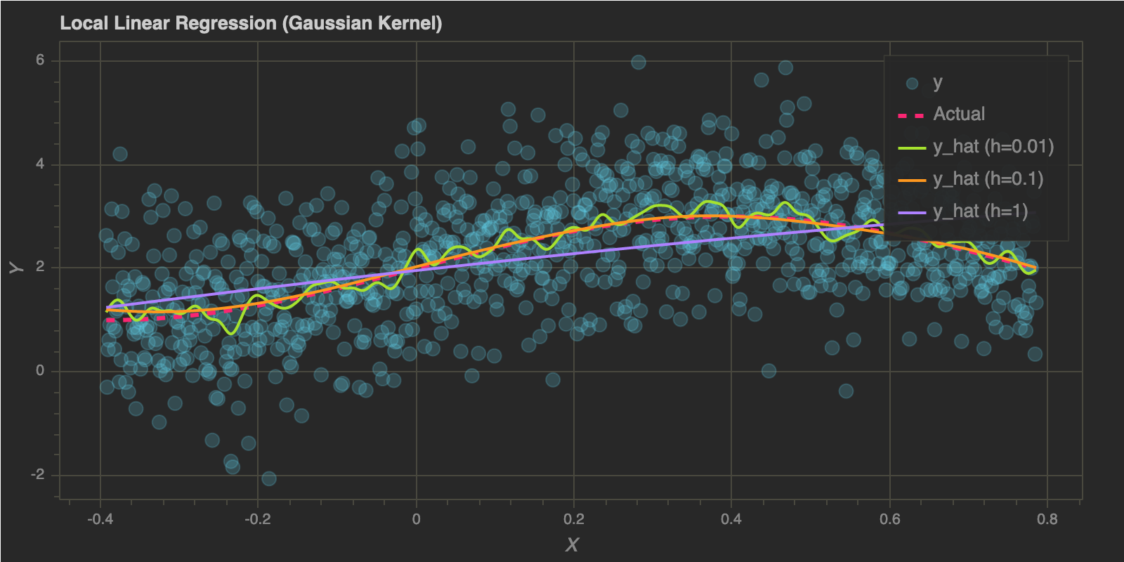
Let’s choose a few bandwidth values and check the fits:

h_values = [0.01, 0.1, 1]
colors = ["#A6E22E", "#FD971F", "#AE81FF"]

p = figure(plot_width=800, plot_height=400)
p.circle(x, y, size=10, alpha=0.2, color="#66D9EF", legend="y")
p.line(x, f(x, 2), color="#F92672", line_width=3, legend="Actual", line_dash="dashed")

for idx, h in enumerate(h_values):
    p.line(x, predict(x, x, y, h), color=colors[idx], line_width=2, legend="y_hat (h={})".format(h))
    
p.title.text = "Local Linear Regression (Gaussian Kernel)"
p.xaxis.axis_label = "X"
p.yaxis.axis_label = "Y"

curdoc().clear()
doc = curdoc()
doc.theme = plot_theme
doc.add_root(p)
show(p)

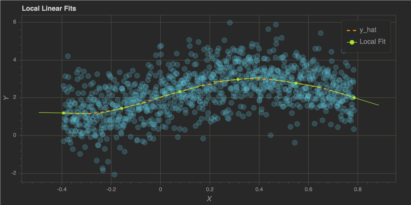
To illustrate how the algorithm works, I wil choose a few $x$ values and show the local linear fits for each of those points. I will use h = 0.1 since the corresponding fit looks pretty reasonable. As explained above, we will get the corresponding $\hat \alpha(x_0)$ and $\hat \beta(x_0)$ for each point.

h_trial = 0.1
x_trials = np.linspace(domain[0], domain[1], 6)

def local_coeffs(x_0, x_train, y_train, h):
    if len(x_train) != len(y_train):
        raise ValueError("X and Y Should have same length")
    
    B = np.array([np.ones(len(x_train)), x_train]).T
    W = np.diag(gaussian_kernel(x_train , x_0, h_trial))
    return np.linalg.inv(B.T.dot(W).dot(B)).dot(B.T).dot(W).dot(y_train)

coeffs = [local_coeffs(x_0, x, y, h_trial) for x_0 in x_trials]
print(coeffs)

[array([ 1.10375711, -0.24977984]), 
array([ 1.93831019,  3.12814681]), 
array([ 2.04711505,  3.62427698]), 
array([ 2.58841427,  1.23608707]), 
array([ 3.96096982, -2.14935988]), 
array([ 5.16166187, -4.00951684])]

Now that we have the local coefficients, let’s plot the local lines at each point in x_trial and the complete fit.

p = figure(plot_width=800, plot_height=400)
p.circle(x, y, size=10, alpha=0.2, color="#66D9EF")

x_left = []
x_right = []
y_left = []
y_right = []

y_fits = []

for cs, x_0 in zip(coeffs, x_trials):
    x_left.append(x_0 - 0.1)
    x_right.append(x_0 + 0.1)
    y_left.append(np.array([1, x_0 - 0.1]).dot(cs))
    y_right.append(np.array([1, x_0 + 0.1]).dot(cs))
    y_fits.append(np.array([1, x_0]).dot(cs))
    

p.line(x, predict(x, x, y, h_trial), color="#FD971F", line_width=2, line_dash="dashed", legend="y_hat")
p.segment(x0=x_left, y0=y_left, x1=x_right, y1=y_right, color="#A6E22E", line_width=1, legend="Local Fit")
p.circle(x_trials, y_fits, size=5, color="#A6E22E", legend="Local Fit")
    
p.title.text = "Local Linear Fits"
p.xaxis.axis_label = "X"
p.yaxis.axis_label = "Y"

curdoc().clear()
doc = curdoc()
doc.theme = plot_theme
doc.add_root(p)
show(p)

One great resource that I came across related to local linear regression is the lecture below (Statistical Machine Learning, Larry Wasserman, CMU, Jan 2016):

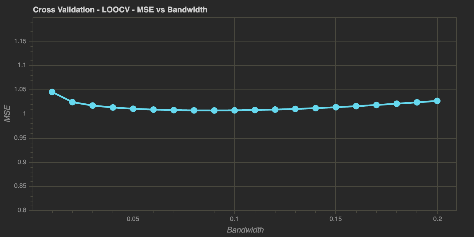
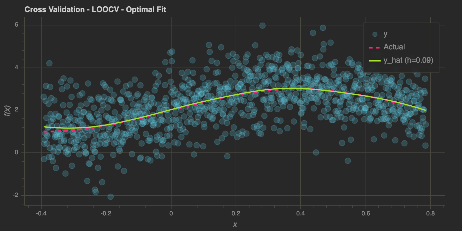
As in the previous post, I will end this post by estimating optimal bandwidth using Leave One Out Cross Validation and K-Fold Cross Validation below:

Cross Validation

Leave One Out Cross Validation (LOOCV)

h_range = np.linspace(0.01, 0.2, 20) # Range to check h in

h_optimal : 0.09

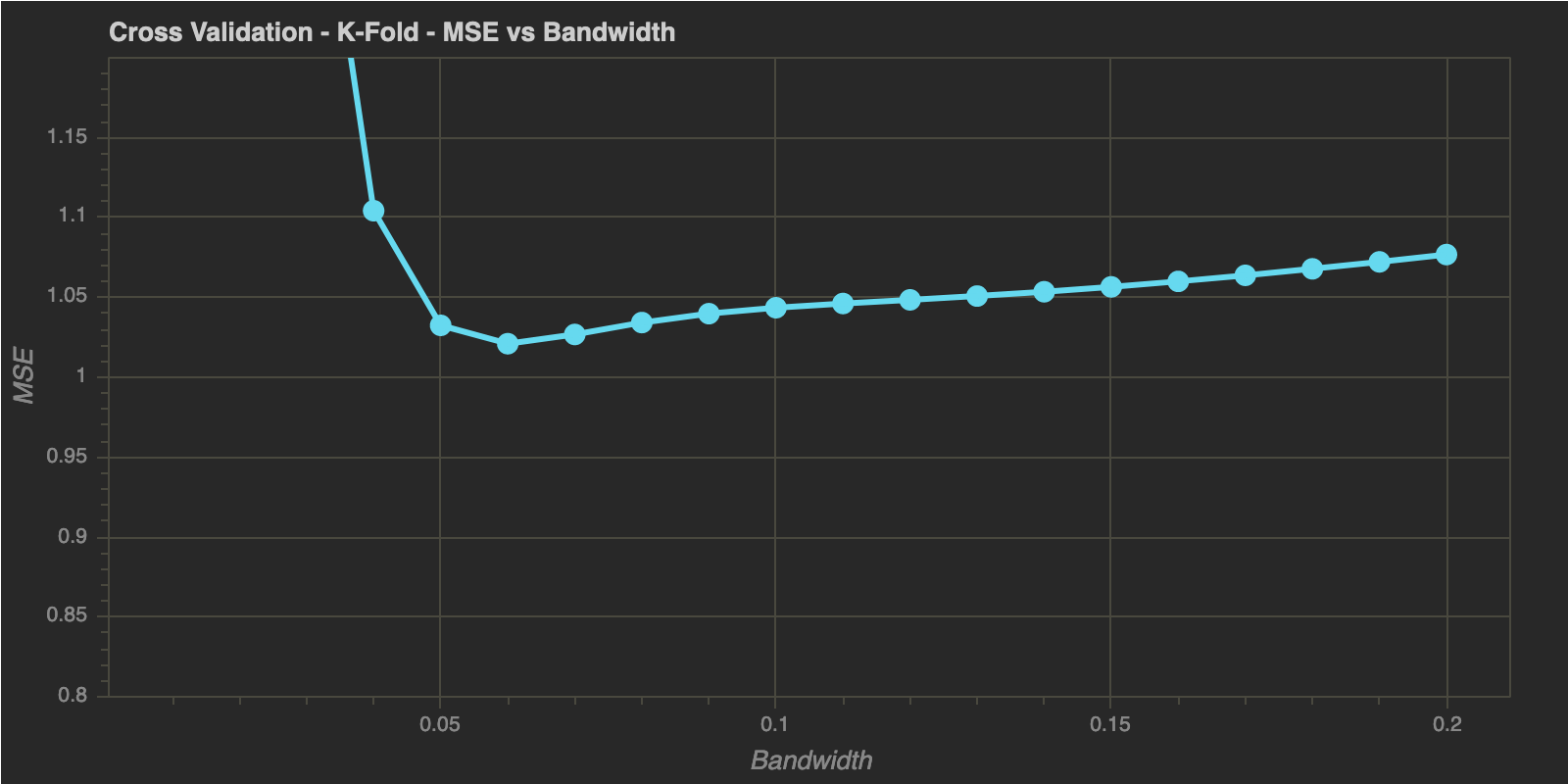
K-Fold Cross Validation

num_folds = 10
num_tries = 5

h_optimal : 0.06

Final Words

In this post, we extended the Kernel Smoothing technique to fit local linear functions instead of local constants at each input point. Fitting locally linear functions helps us reduce the bias and error on the edges and sparse regions of our data.

Sources

1. Elements of Statistical Learning - Chapter 6
2. Non-Parametric regression