Kernel Smoothing

Kernel Method is one of the most popular non-parametric methods to estimate probability density and regression functions. As the word Non-Parametric implies, it uses the structural information in the existing data to estimate response variable for out-of-sample data.

In this post, I will go through an example to estimate a simple non-linear function using Gaussian Kernel smoothing from first principles. I will also discuss how to use Leave One Out Cross Validation (LOOCV) and K-Fold Cross Validation to estimate the bandwidth parameter \(h\) for the kernel.

Setup

Let’s setup our environment.

Also, I have a Jupyter notebook for this post on my Github.

import numpy as np
import pandas as pd

from bokeh.io import output_notebook, push_notebook, curdoc, output_file
from bokeh.plotting import figure, show
from bokeh.themes import Theme
from bokeh.embed import components

Here’s a handy trick if you want to use your own theme in bokeh. I have added the theme below in the Appendix.

plot_theme = Theme("./theme.yml") 
# Use it like this: 
# doc = curdoc()
# doc.theme = plot_theme
# doc.add_root(p)

Sample Data

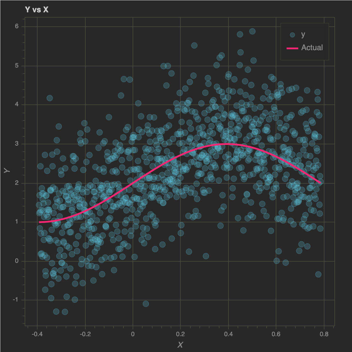
Let’s generate some data for fitting. I will use the function \(\mathbf{y = f(x) = sin(4x)}\)

def f(x, c):
    return np.sin(4 * x) + c

data_size = 1000
domain = (-np.pi/8, np.pi/4)
std = 1.0
const = 2.0
x = np.linspace(domain[0], domain[1], data_size)
y = f(x, const) + np.random.normal(0, std, data_size)

Let’s do a scatter plot of the data:

p = figure(plot_width=600, plot_height=600)
p.circle(x, y, size=10, alpha=0.2, color="#66D9EF", legend="y")
p.line(x, f(x, 2), color="#F92672", line_width=3, legend="Actual")

p.title.text = "Y vs X"
p.xaxis.axis_label = "X"
p.yaxis.axis_label = "Y"

curdoc().clear()
doc = curdoc()
doc.theme = plot_theme
doc.add_root(p)
show(p)

Smoothing

Gaussian Kernel

Gaussian Kernel or Radial Basis Function Kernel is a very popular kernel used in various machine learning techniques. The kernel is given by:

\begin{equation} \mathbf{K(x, x_0)} = exp( - \dfrac{||x - x_0||^2}{2 h^2}) \end{equation}

\(h\) is a free parameter also called the bandwidth parameter. It determines the width of the kernel.

def gaussian_kernel(x, x0, h):
    return np.exp(- 0.5 * np.power((x - x0) / h, 2) )

One Dimentional Smoother

In Kernel Regression, for a given point \(x_0\), we use a weighted average of the nearby points’ response variable as the estimated value. One such technique is k-Nearest Neighbor Regression.

In Kernel Smoothing, we take the idea further by using all the training data and continously decrease the weights for points farther away from the given point \(x_0\). The bandwidth parameter \(h\) mentioned earlier controls the decreasing rate of the weights. Bandwidth \(h\) can also be interpreted as the width of the kernel, centered at \(x_0\).

When the bandwidth is smaller, the weighting effect of the kernel is more localized

This idea of localization goes beyond Gaussian Kernel and also applies to other common kernel functions such as the Epanechnikov Kernel.

As part of the procedure, we use the kernel function and the bandwidth \(h\) to smooth the data points to obtain a local estimate of the response variable.

The final estimator is given by:

\begin{equation} \mathbf{\hat f(x_0)} = \mathbf{\hat y_i} = \dfrac{\sum_{i=1}^{N} K_h(x_0, x_i) y_i}{\sum_{i=1}^{N} K_h(x_0, x_i)} \end{equation}

where \(\mathbf{K_h}\) represents kernel with a specific bandwidth \(h\).

In essense, it is the weighted average of all the response variable values \(y_i\) with weights equal to the kernel function centered at \(x_0\) (the estimation point) for each \(x_i\). Different bandwidth values will give different kernel function values, and in turn, different weights.

Let’s implement it in Python to see the results of changing the bandwidth:

def predict(x_test, x_train, y_train, bandwidth, kernel_func=gaussian_kernel):
    return np.array([(kernel_func(x_train, x0, bandwidth).dot(y_train) ) / 
                     kernel_func(x_train, x0, bandwidth).sum() for x0 in x_test])

h_values = [0.01, 0.1, 1]
colors = ["#A6E22E", "#FD971F", "#AE81FF"]

p = figure(plot_width=600, plot_height=600)
p.circle(x, y, size=10, alpha=0.2, color="#66D9EF", legend="y")
p.line(x, f(x, 2), color="#F92672", line_width=3, legend="Actual", line_dash="dashed")

for idx, h in enumerate(h_values):
    p.line(x, predict(x, x, y, h), color=colors[idx], line_width=2, legend="y_hat (h={})".format(h))
    
p.title.text = "Kernel Regression (Gaussian)"
p.xaxis.axis_label = "X"
p.yaxis.axis_label = "Y"

curdoc().clear()
doc = curdoc()
doc.theme = plot_theme
doc.add_root(p)
show(p)

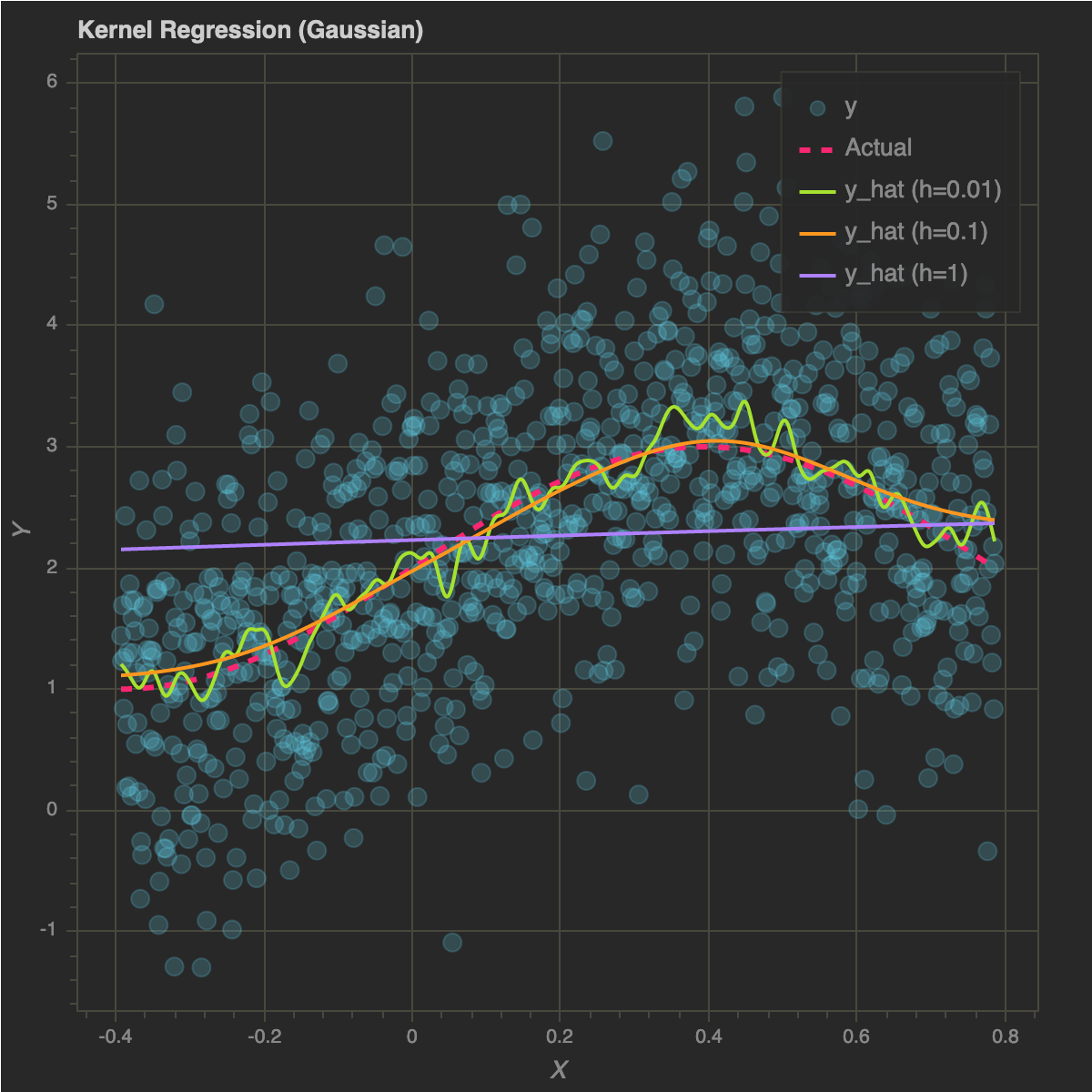
As seen from the estimators for different \(h\), kernel smoothing suffers from the Bias-Variance Tradeoff:

• As \(h\) decreases, variance of the estimates gets larger, bias gets smaller, and the effect of the kernel is localized
• As \(h\) increases, variance of the estimates gets smaller, bias gets larger, and the effect of the kernel is spread out

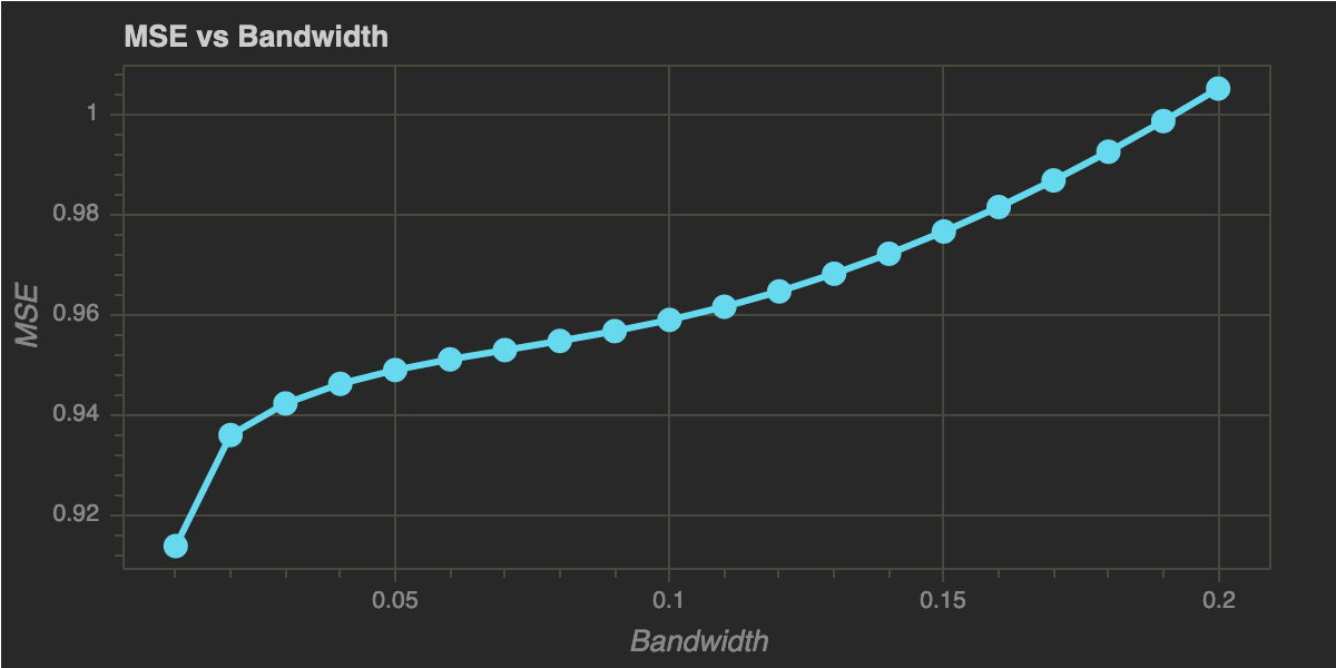
Let’s plot the Mean Squared Error MSE of the estimates versus the bandwidth:

h_range = np.linspace(0.01, 0.2, 20)

mses = [np.mean(np.power(y - predict(x, x, y, h), 2)) for h in h_range]

p = figure(plot_width=600, plot_height=300)
p.circle(x=h_range, y=mses, size=10, color="#66D9EF")
p.line(x=h_range, y=mses, color="#66D9EF", line_width=3)

p.title.text = "MSE vs Bandwidth"
p.xaxis.axis_label = "Bandwidth"
p.yaxis.axis_label = "MSE"

curdoc().clear()
doc = curdoc()
doc.theme = plot_theme
doc.add_root(p)
show(p)

The next step is to find a “good” value for bandwidth and we can use Cross Validation for that.

Cross Validation

Cross Validation is a common method to tackle over-fitting the parameters of the model. The data is split into parts such that some of it is used as the training set and the rest as the validation set.

Splitting the data helps with not using the same data twice to fit the model parameters. Either the data point is used in training set or validation set. Training set is used to fit our model parameters, which are used to predict the values of response variable in the validation set. Hence, we can calculate the quality of our prediction based on the prediction error of validation set.

scikit-learn has modules for different cross validation techniques. However, I will implement these from scratch using numpy to avoid the dependency on scikit-learn just for cross validation.

Let’s discuss two of these techniques:

Leave One Out Cross Validation (LOOCV)

In Leave One Out Cross Validation (LOOCV), we leave one observation out as the validation set and the remaining data points are used for model building. Finally, the response variable is predicted for the left out value as the validation set.

mse_values = []

for h in h_range:
    errors = []
    for idx, val in enumerate(x):
        x_test = np.array([val])
        y_test = np.array([y[idx]])
        x_train = np.append(x[:idx], x[idx+1:])
        y_train = np.append(y[:idx], y[idx+1:])
        assert len(x_train) == data_size - 1
        y_test_hat = predict(x_test, x_train, y_train, h)
        errors.append((y_test_hat - y_test)[0])
    mse_values.append(np.mean(np.power(errors, 2)))

Let’s plot the Mean Squared Error MSE of the estimates versus the bandwidth, as earlier:

p = figure(plot_width=600, plot_height=300)
p.circle(x=h_range, y=mse_values, size=10, color="#66D9EF")
p.line(x=h_range, y=mse_values, color="#66D9EF", line_width=3)

p.title.text = "Cross Validation - LOOCV - MSE vs Bandwidth"
p.xaxis.axis_label = "Bandwidth"
p.yaxis.axis_label = "MSE"

curdoc().clear()
doc = curdoc()
doc.theme = plot_theme
doc.add_root(p)
show(p)

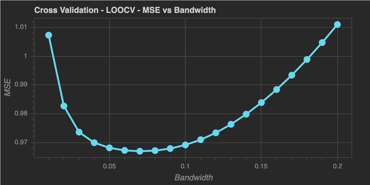
As we can see, we can find an optimal bandwidth value to minimize the MSE. Let’s check the fit for that bandwidth:

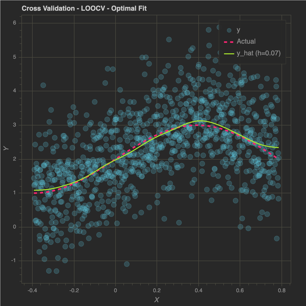
h_optimal = h_range[np.argmin(mse_values)]
print(h_optimal)

# Output:
# 0.07

Below the estimator for the optimal bandwidth \(0.07\):

p = figure(plot_width=600, plot_height=600)
p.circle(x, y, size=10, alpha=0.2, color="#66D9EF", legend="y")
p.line(x, f(x, 2), color="#F92672", line_width=3, legend="Actual", line_dash="dashed")

p.line(x, predict(x, x, y, h_optimal), color="#A6E22E", line_width=2, legend="y_hat (h={})".format(h_optimal))
    
p.title.text = "Cross Validation - LOOCV - Optimal Fit"
p.xaxis.axis_label = "X"
p.yaxis.axis_label = "Y"

curdoc().clear()
doc = curdoc()
doc.theme = plot_theme
doc.add_root(p)
show(p)

K-Fold Cross Validation

Another popular cross validation technique is K-Fold Cross Validation, where data is divided in \(K\) random chunks. One of the chunks is used as the validation set and the rest as the training set. This procedure is repeated several times to get the prediction error for each value of bandwidth.

Here is an implementation of K-Fold CV:

def split_k_fold(x, y, folds):
    if len(x) != len(y):
        raise ValueError("X and Y Should have same length")
    indices = np.arange(len(x))
    np.random.shuffle(indices)
    split_size = len(x) // folds
    return np.array([x[n * split_size:(n + 1) * split_size] for n in np.arange(folds)]), np.array(
        [y[n * split_size:(n + 1) * split_size] for n in np.arange(folds)])

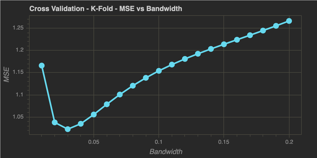
Let’s try \(K = 4\) and \(10\) tries for each \(h\). Similar to LOOCV, let’s plot the MSE vs bandwidth to see their relationship. Again, we can optimize the bandwidth by minimizing the MSE.

num_folds = 4
num_tries = 10

fold_indices  = np.arange(num_folds)
mse_values = []

for h in h_range:
    trial_mses = []
    for trial in np.arange(num_tries):
        x_splits, y_splits = split_k_fold(x, y, num_folds)
        mses = []
        for idx in fold_indices:
            test_idx = idx
            train_idx = np.setdiff1d(fold_indices, [idx])
            train_x, test_x, train_y, test_y = (np.concatenate(x_splits[train_idx]), 
                                                x_splits[test_idx], 
                                                np.concatenate(y_splits[train_idx]), 
                                                y_splits[test_idx])
            test_y_hat = predict(test_x, train_x, train_y, h)
            mses.append(np.mean(np.power(test_y_hat - test_y, 2)))
        trial_mses.append(np.mean(mses))
    mse_values.append(np.mean(trial_mses))

p = figure(plot_width=600, plot_height=300)
p.circle(x=h_range, y=mse_values, size=10, color="#66D9EF")
p.line(x=h_range, y=mse_values, color="#66D9EF", line_width=3)

p.title.text = "Cross Validation - K-Fold - MSE vs Bandwidth"
p.xaxis.axis_label = "Bandwidth"
p.yaxis.axis_label = "MSE"

curdoc().clear()
doc = curdoc()
doc.theme = plot_theme
doc.add_root(p)
show(p)

h_optimal = h_range[np.argmin(mse_values)]
print(h_optimal)

# Output:
# 0.03

p = figure(plot_width=600, plot_height=600)
p.circle(x, y, size=10, alpha=0.2, color="#66D9EF", legend="y")
p.line(x, f(x, 2), color="#F92672", line_width=3, legend="Actual", line_dash="dashed")

p.line(x, predict(x, x, y, h_optimal), color="#A6E22E", line_width=2, legend="y_hat (h={})".format(h_optimal))
    
p.title.text = "Cross Validation - K-Fold - Optimal Fit"
p.xaxis.axis_label = "X"
p.yaxis.axis_label = "Y"

curdoc().clear()
doc = curdoc()
doc.theme = plot_theme

doc.add_root(p)
show(p)

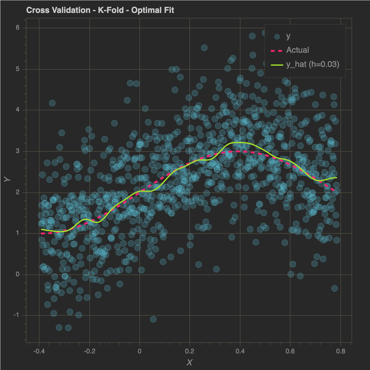
For this particular example, compared to LOOCV, K-Fold CV smoothing is more localized as it has a lower value of bandwidth. However, both approaches show a similar releationship between MSE and bandwidth.

Disadvantages of Kernel Smoothing

• Weights calculated at the boundaries are biased due to one side of the kernel being cut off. This leads to biased estimates at the boundaries.
• Issues can also arise if the data is not spacially uniform. Spaces with fewer data points will have more biased estimates since there will be fewer nearby points to weight the response variable values.

Final Words

In this post, we took a step-by-step approach to fit Kernel Smoothing using Gaussian Kernel. Same approach can be applied using other kernels. We also applied Cross Validation to choose an optimal bandwidth parameter.

Sources

1. Elements of Statistical Learning - Chapter 6
2. Stanford STATS 306

Appendix

Bokeh Theme

### Monokai-inspired Bokeh Theme
# written July 23, 2017 by Luke Canavan

### Here are some Monokai palette colors for Glyph styling
# @yellow: "#E6DB74"
# @blue: "#66D9EF"
# @pink: "#F92672"
# @purple: "#AE81FF"
# @brown: "#75715E"
# @orange: "#FD971F"
# @light-orange: "#FFD569"
# @green: "#A6E22E"
# @sea-green: "#529B2F"

attrs:
    Axis:
        axis_line_color: "#49483E"
        axis_label_text_color: "#888888"
        major_label_text_color: "#888888"
        major_tick_line_color: "#49483E"
        minor_tick_line_color: "#49483E"
    Grid:
        grid_line_color: "#49483E"
    Legend:
        border_line_color: "#49483E"
        background_fill_color: "#282828"
        label_text_color: "#888888"
    Plot:
        background_fill_color: "#282828"
        border_fill_color: "#282828"
        outline_line_color: "#49483E"
    Title:
        text_color: "#CCCCCC"