Geometry of Regression

A picture is worth a thousand words. This post on stats Stack Exchange gives a great description of the geometric representation of Linear Regression problems. Let’s see this in action using some simple examples.

The below graphic, which appeared in the original stack-exchange post, captures the essence of Linear Regression very aptly.

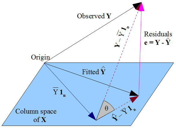
Source: Stack Exchange

Overview

The geometrical meaning of the Linear/Multiple Regression fit is the projection of predicted variable $y$ on $\mathbf{span(1, X)}$ (with constant) or $\mathbf{X}$ (without constant).

In terms of more generally understood form of Linear Regression:

• With Constant: $\hat y = \beta_o + \beta_1 x$
• Without Constant: $\hat y = \beta_1 x$

We will focus on regression with constant.

Regression coefficients represent the factors that make a linear combination of $\mathbb{1}$ and $\mathbf{X}$ i.e. the projection of $y$ in terms of a linear combination of $\mathbb{1}$ and $\mathbf{X}$.

Additionally, $\mathbf{N}$ data points imply an $\mathbf{N}$-dimensional vector for $y$, $\mathbb{1}$, and $\mathbf{X}$. Hence, I will be using only three data points for predictor and predicted variables to restrict ourselves to 3 dimensions. Reader can create the above graphic using the analysis below if they wish.

Analysis

import numpy as np
import matplotlib.pyplot as plt
import sympy as sp

%matplotlib inline
sp.init_printing(use_unicode=True)
plt.style.use("ggplot")

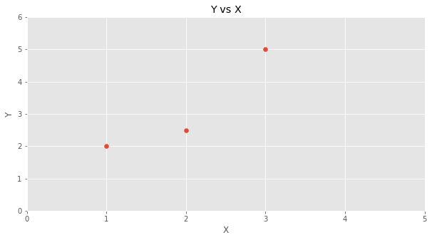
Let’s create our $y$ and $\mathbf{X}$.

x = np.array([1.0, 2, 3])
y = np.array([2, 2.5, 5])

Y = sp.Matrix(y)
Y

\[\left[\begin{matrix}2.0\\2.5\\5.0\end{matrix}\right]\]

X = sp.Matrix(np.transpose([np.ones(len(x)), x]))
X

\[\left[\begin{matrix}1.0 & 1.0\\1.0 & 2.0\\1.0 & 3.0\end{matrix}\right]\]

fig = plt.figure()
plt.scatter(X.col(1), y)
plt.xlim((0, 5))
plt.ylim((0, 6))
plt.title("Y vs X")
plt.xlabel("X")
plt.ylabel("Y")
plt.gcf().set_size_inches(10, 5)
plt.show()

Regression Coefficients

Linear regression coefficients $\beta$ are given by:

\begin{equation} \beta = (\mathbf{X^\intercal} \mathbf{X})^{-1} \mathbf{X^\intercal} y \end{equation}

Let’s calculate $\mathbf{\beta}$ for $\mathbf{X}$ and $y$ we defined above.

beta = ((X.transpose() * X) ** -1) * X.transpose() * y
beta

\[\left[\begin{matrix}0.166666666666668\\1.5\end{matrix}\right]\]

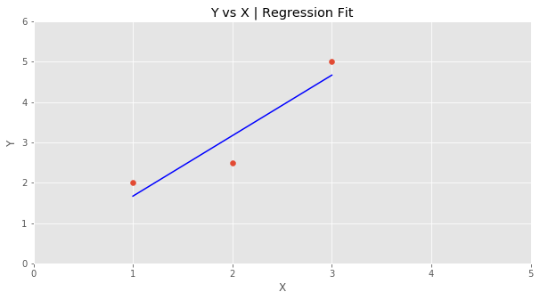
Since we now have $\beta$, we can calculate the estimated $y$ or $\hat y$.

\begin{equation} \hat y = \mathbf{X} \beta = \mathbf{X} (\mathbf{X^\intercal} \mathbf{X})^{-1} \mathbf{X^\intercal} y \end{equation}

y_hat = X * beta
y_hat

\[\left[\begin{matrix}1.66666666666667\\3.16666666666667\\4.66666666666667\end{matrix}\right]\]

fig = plt.figure()
plt.scatter(x, y)
plt.xlim((0, 5))
plt.ylim((0, 6))
plt.title("Y vs X | Regression Fit")
plt.xlabel("X")
plt.ylabel("Y")
plt.plot(X.col(1), y_hat, color='blue')
plt.gcf().set_size_inches(10, 5)
plt.show()

Error Analysis

Residuals for the model are given by: $\epsilon$ = $\hat y$ - $y$. This represents the error in predicted values of $y$ using both $\mathbb{1}$ and $\mathbf{X}$ in the model. The error vector is normal to the $\mathbf{span(1, X)}$ since it represents the component of $y$ that is not in $\mathbf{span(1, X)}$.

res = y - y_hat
res

\[\left[\begin{matrix}0.333333333333332\\-0.666666666666668\\0.333333333333332\end{matrix}\right]\]

Average vector or $\bar y$ is geometrically the projection of $y$ on just the $\mathbb{1}$ vector.

y_bar = np.mean(y) * sp.Matrix(np.ones(len(y)))
y_bar

\[\left[\begin{matrix}3.16666666666667\\3.16666666666667\\3.16666666666667\end{matrix}\right]\]

We can calculate the error in the average model or where we represent the predicted values as the average vector $\bar y$. Error in the model is given by $\kappa$ = $\bar y$ - $y$.

kappa = y_bar - y
kappa

\[\left[\begin{matrix}1.16666666666667\\0.666666666666667\\-1.83333333333333\end{matrix}\right]\]

Both $\bar y$ and $\hat y$ are predictors for $y$ and it is reasonable to calculate how much error we reduce by adding $\mathbf{X}$ to the model. Let’s call the error $\eta$

eta = y_hat - y_bar
eta

\[\left[\begin{matrix}-1.5\\1.77635683940025 \cdot 10^{-15}\\1.5\end{matrix}\right]\]

Now from here we can prove whether $\eta$ and $\epsilon$ are perpendicular to each other. We can check it by calculating their dot product.

dot_product = eta.transpose() * res
dot_product

\[\left[\begin{matrix}5.55111512312578 \cdot 10^{-16}\end{matrix}\right]\]

Hence, we can see that $\eta$ and $\epsilon$ are normal to each other since their dot product is 0

From here we can also prove the relationship between Total Sum of Squares (SST), Sum of Squares due to Squares of Regression (SSR) and Sum of Squares due to Squares of Errors (SSE)

$\mathbf{SST} = \mathbf{SSR} + \mathbf{SSE}$

• $\mathbf{SST}$ can be represented by the squared norm of $\kappa$
• $\mathbf{SSR}$ can be represented by the squared norm of $\eta$
• $\mathbf{SSE}$ can be represented by the squared norm of $\epsilon$

We can use Pythagorean Theorem to check the above relationship i.e. \begin{equation} ||\kappa||^2 = ||\eta||^2 + ||\epsilon||^2 \end{equation}

kappa.norm() ** 2  - eta.norm() ** 2 - res.norm() ** 2

\[1.66533453693773 \cdot 10^{-15}\]

Hence, as we expected, $\kappa$, $\eta$ and $\epsilon$ form a right angled triangle.

Summary

Through this post, I demonstrated how we can interpret linear/multiple regression geometrically.

Also, I solved a linear regression model using Linear Algebra.